学习 Andrej Karpathy 的 micrograd 项目,从零开始实现一个自动微分框架,深入理解反向传播和链式法则的核心原理。
从 0 实现一个极简的自动微分框架
代码仓库:https://github.com/karpathy/nn-zero-to-hero
Andrej Karpathy 是著名深度学习课程 Stanford CS 231n 的作者与主讲师,也是 OpenAI 创始人之一,“micrograd” 是他创建的一个小型、教育性质的项目。这个项目实现了一个非常简化的自动微分和梯度下降库,学习者只需要拥有最基本的微积分知识即可,用于教学和演示目的。
Micrograd 介绍
Micrograd 基本上是一个autograd(自动梯度) 引擎,它的真正作用是实现反向传播。
反向传播是一种算法,可以有效地计算神经网络中某种损失函数相对于权重的梯度。这让我们能够迭代地调整神经网络的权重,以最小化损失函数,从而提高网络的准确性。因此,反向传播将成为任何现代深度神经网络库 (如 PyTorch、JAX) 的数学核心。
micrograd 支持的操作种类:
from micrograd.engine import Value
a = Value(-4.0)
b = Value(2.0)
c = a + b # C 的字节点是 A 和 B,因为 C 维护 A 和 B 值对象的指针
d = a * b + b**3
c += c + 1
c += 1 + c + (-a)
d += d * 2 + (b + a).relu()
d += 3 * d + (b - a).relu()
e = c - d
f = e**2
g = f / 2.0
g += 10.0 / f # 前向传递的输出
print(f'{g.data:.4f}') # prints 24.7041, the outcome of this forward pass
g.backward() # 在节点 G 处初始化反向传播,从微积分中递归地引用链式法则,可以评估 G 相对于所有内部节点的导数
print(f'{a.grad:.4f}') # prints 138.8338, i.e. the numerical value of dg/da
print(f'{b.grad:.4f}') # prints 645.5773, i.e. the numerical value of dg/db这会告诉我们,如果对 A 和 B 进行微小的正向调整,G 会如何响应。
可以看出,实现这些操作的重点在于Value类的实现方式,下面将详细介绍实现思路。
神经网络原理
基本来说,神经网络只是数学表达式,他们将输入数据作为输入,将神经网络的权重作为输入,输出的就是神经网络的预测结果或损失函数。
这里的引擎是在单个标量的级别上工作,分解到这些原子操作和所有的加号、乘号,这是有些过度的。你永远不会再生产环境中执行这些操作,这里做的只是为了教学目的,因为它不需要处理现代深度神经网络库中使用的 n 维张量 (nd tensor)。这样做只是为了让你理解并重构反向传播和链式法则,以及神经网络训练的理解。如果要训练更大的神经网络,则必须使用这些张量,但数学方式并没有改变。
导数的理解
import numpy as np
import matplotlib.pyplot as plt
import math
%matplotlib inline# Define a scalar function f(x), which accepts a scalar x and returns a scalar y
def f(x):
return 3*x**2 - 4*x + 5
f(3.0)20.0
# Create a set of scalar values to feed into f(x)
xs = np.arange(-5, 5, 0.25)
'''
xs = array([-5. , -4.75, -4.5 , -4.25, -4. , -3.75, -3.5 , -3.25, -3. ,
-2.75, -2.5 , -2.25, -2. , -1.75, -1.5 , -1.25, -1. , -0.75,
-0.5 , -0.25, 0. , 0.25, 0.5 , 0.75, 1. , 1.25, 1.5 ,
1.75, 2. , 2.25, 2.5 , 2.75, 3. , 3.25, 3.5 , 3.75,
4. , 4.25, 4.5 , 4.75])
'''
# Apply f(x) to each value in xs
ys = f(xs)
'''
ys = array([100. , 91.6875, 83.75 , 76.1875, 69. , 62.1875,
55.75 , 49.6875, 44. , 38.6875, 33.75 , 29.1875,
25. , 21.1875, 17.75 , 14.6875, 12. , 9.6875,
7.75 , 6.1875, 5. , 4.1875, 3.75 , 3.6875,
4. , 4.6875, 5.75 , 7.1875, 9. , 11.1875,
13.75 , 16.6875, 20. , 23.6875, 27.75 , 32.1875,
37. , 42.1875, 47.75 , 53.6875])
'''
# Plot the results
plt.plot(xs, ys)
图上每个 x 的导数是多少?
OFC,f’(x) = 6x - 4,但我们不会这样做,因为在神经网络中没有人会真正写出表达式。
这将是一个庞大的表达式,所以我们不会采取这种符号化的方法。
导数的定义
相反,让我们来看一下导数的定义,确保我们真正理解它。
# We can basically evaluate the derivate here numerically by taking a very small h
h = 0.00000001
x = 3.0
(f(x + h) - f(x)) / h # the function respond positively14.00000009255109
这是函数在正方向上的响应。
After normalization by the run, So we have the rise over run to get the numerical approximation of the slope(上升/横向移动得到数值近似的斜率)
而在某个位置上,如果我们朝着正方向推进,函数没有响应,几乎保持不变,这就是为什么slope=0
导数能告诉我们什么
看一个更复杂的例子:
a = 2.0
b = -3.0
c = 10
d = a * b + c
print(d)这个函数的输出变量 d 是三个标量输入的函数,我们需要再次审视关于 d 相对于 a、b 和 c 的导数。
h = 0.0001
# inputs
a = 2.0
b = -3.0
c = 10
d1 = a * b + c
a += h
d2 = a * b + c
print('da',d1)
print('d2',d2)
print('slope', (d2 - d1) / h)这里要感悟在推进 a 后,d2 的变化是什么样的
我们发现 a 是正数,b 是负数,a 变大则会减少加到 d 上的内容,所以我们可以预料到函数值 d2 会变小。
da 4.0 d2 3.999699999999999 slope -3.000000000010772
从数学上也可以证明,
b += hda 4.0 d2 4.0002 slope 2.0000000000042206

函数提升的量与我们添加到 c 上的量是相同的,所以斜率是 1
现在我们已经对导数是如何告诉你有关这个函数的信息有了一些直观的感觉,我们可以转向神经网络了。
框架实现
自定义类的数据结构
前面也提到了,神经网络是非常庞大的数学表达式,所以我们需要一些数据结构来维护这些表达式。
class Value:
def __init__(self, data):
self.data = data
def __repr__(self):
return f"Value({self.data})"
def __add__(self, other):
out = Value(self.data + other.data)
return out
def __mul__(self, other):
out = Value(self.data * other.data)
return out
a = Value(2.0)
b = Value(-3.0)
c = Value(10.0)
d = a * b + c # (a.__mul__(b)).__add__(c)
repr的作用是为我们提供一种打印输出的方法
现在我们缺少的是这个表达式的联系组织,我们需要知道并保留有关哪些值产生了哪些其它值的指针。
def __init__(self, data, _children=(), _op=''):
self.data = data
self._prev = set(_children)
self._op = _op
def __repr__(self):
return f"Value({self.data})"
def __add__(self, other):
out = Value(self.data + other.data, (self, other), '+')
return out
def __mul__(self, other):
out = Value(self.data * other.data, (self, other), '*')
return out这样可以知道每个值的子项,并且追到了是哪个运算操作生成了这个值
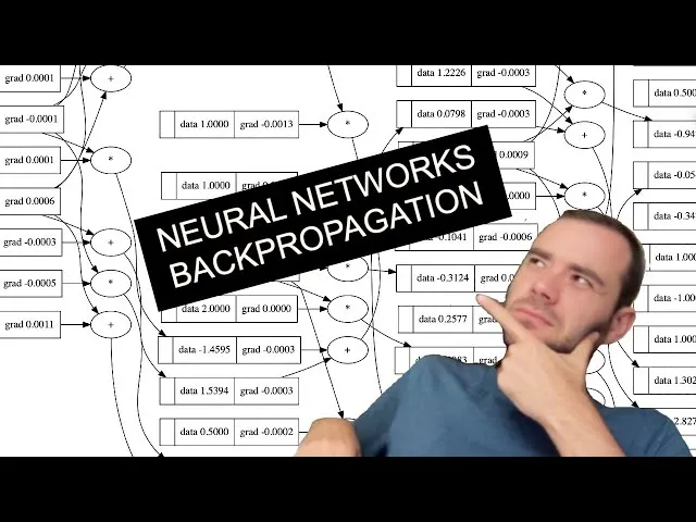
现在我们拥有了完整的数学表达式,需要寻找一个更好的可视化方法来表现会变得很大的表达式。(不是重点,可以跳过)
from graphviz import Digraph
def trace(root):
# builds a set of all node and edges in the graph
nodes, edges = set(), set()
def build(v):
if v not in nodes:
nodes.add(v)
for child in v._prev:
edges.add((child, v))
build(child)
build(root)
return nodes, edges
def draw_dot(root):
dot = Digraph(format='svg', graph_attr={'rankdir': 'LR'}) # LR = left to right
nodes, edges = trace(root)
for n in nodes:
uid = str(id(n))
# for many value in graph, create a rectangular ('record') node for it
dot.node(name = uid, label = "{ %s | data %.4f}" % (n.label, n.data), shape = 'record')
if n._op:
# if this value is a result of some operation, create an op node for it
dot.node(name = uid + n._op, label = n._op)
# and connect this node for it
dot.edge(uid + n._op, uid)
for n1, n2 in edges:
# connect n1 to the op node of n2
dot.edge(str(id(n1)), str(id(n2)) + n2._op)
return dot
draw_dot(d)需要在 Value 类中添加
label成员,并修改定义如下:
a = Value(2.0, label='a')
b = Value(-3.0, label='b')
c = Value(10.0, label='c')
e = a * b; e.label = 'e'
d = e + c; d.label = 'd'
d
现在让表达式更深一层:
f = Value(-2.0, label='f')
L = d * f; L.label = 'L'
L
draw_dot(L)
可视化前向传递
运行反向传播
我们将从 L 开始,反向计算沿着所有中间值的梯度。在神经网络环境中,你会对神经网络的权重相对于损失函数 L 的导数非常感兴趣。
在 Value 类汇总创建一个变量来维护关于该值的 L 的导数:
self.grad = 0在初始化时,我们假设每个值都不会影响输出。因为导数为 0 意味着这个变量不会改变损失函数。
现在我们从 L 开始填写梯度,那么 L 关于 L 的导数是多少?换言之,如果我把 L 变为一个微小的量 h,L 会变化多少?
不难想出,L 会随着 h 的变化而成比例变化,因此导数为 1:
def lol():
h = 0.0001
a = Value(2.0, label='a')
b = Value(-3.0, label='b')
c = Value(10.0, label='c')
e = a * b; e.label = 'e'
d = e + c; d.label = 'd'
f = Value(-2.0, label='f')
L = d * f; L.label = 'L'
L1 = L.data
a = Value(2.0, label='a')
b = Value(-3.0, label='b')
c = Value(10.0, label='c')
e = a * b; e.label = 'e'
d = e + c; d.label = 'd'
f = Value(-2.0, label='f')
L = d * f; L.label = 'L'
L2 = L.data + h
print((L2 - L1) / h)
lol() # 0.9999999999976694L.grad = 1.0
# L = d * f
# dL/dd = ? -> f
f.grad = 4.0 # d.data
d.grad = -2.0 # f.data我们通过lol()函数所做的有点像时一个内链梯度检查,也就是我们在进行反向传播并获取相对于所有中间结果的导数时所进行的操作。数值梯度仅仅是使用小步长来估计它。
现在我们开始进入反向传播的要点,我们知道 L 对 D 很敏感,但是 L 如何受到 C 的影响呢?
'''
dd / dc = ? -> 1.0 得到局部导数
dd / de = ? -> 1.0
d = c + e
(f(x+h)) - f(x) / h
((c + h + e) - (c + e)) / h
h / h = 1.0
'''计算local derivate
c、e、d 中间的+节点完全不知道全图的其余部分,它只知道自己做了一个 add 操作并 created d,以及 c、e 对 d 的局部影响,不过我们实际想要的是 dL/dc。
我们怎么将这些信息整合在一起以得到 dL/dc 呢?答案是微积分中的Chain Rule 链式法则
如果变量 z 依赖于变量 y,而变量 y 又依赖于变量 x(即 y 和 z 是因变量),那么 z 也通过中间变量 y 来依赖于 x。在这种情况下,链式法则可以表示为:
链式法则基本上告诉你如何正确地将这些导数链接在一起
正如乔治·F·西蒙斯所说:“如果一辆汽车的速度是自行车的两倍,而自行车的速度是步行者的四倍,那么汽车比人快 8 倍。”
这个例子很明白的解释了这个法则的核心,也就是Multiply
加法节点
distributor of gradient
在神经网络中,每个节点的操作都会对梯度的传播方式产生影响。对于加法节点,假设有两个输入 和 ,它们相加得到 。在反向传播过程中, 相对于 和 的梯度分别是 1。
具体来说:
- 如果 的梯度是 ,其中 是损失函数,那么根据链式法则,我们可以得到 和 的梯度:
- 由于 ,因此 和 。
- 因此, 和 都等于 。
所以,在加法节点,梯度会被”原样”传递给所有输入节点。这意味着加法节点不会改变梯度的大小,而是将梯度均匀分配给所有输入。这是因为加法操作对于每个输入来说是线性的,并且每个输入对输出的贡献是独立的。
乘法节点
若想求a.grad,可由:
所以反向传播核心思想可以概括为:递归乘以局部导数 recursively multiply on the local derivatives
微调输入
微调输入,尝试让 L 值增加。
对 a 点操作的话,意味着我们只需要朝着梯度方向前进。 我们需要对叶子节点进行调整,因为通常情况下,我们对它们有控制权。 我们期待 L 会升高:
a.data += 0.01 * a.grad
b.data += 0.01 * b.grad
c.data += 0.01 * c.grad
f.data += 0.01 * f.grad
e = a * b
d = e + c
L = d * f
print(L.data)-7.286496
使用一个实际的例子:
# inputs x1,x2
x1 = Value(2.0, label='x1')
x2 = Value(0.0, label='x2')
# weights w1,w2, 每个输入的突触强度
w1 = Value(-3.0, label='w1')
w2 = Value(1.0, label='w2')
# bias b 偏置
b = Value(6.8813735870195432, label='b')
# x1*w1 + x2*w2 + b
x1w1 = x1 * w1; x1w1.label = 'x1w1'
x2w2 = x2 * w2; x2w2.label = 'x2w2'
x1w1x2w2 = x1w1 + x2w2; x1w1x2w2.label = 'x1w1x2w2'
n = x1w1x2w2 + b; n.label = 'n' # 细胞体的原始激活值# 现在用一个激活函数来处理,这里使用 tanh,在先前的类中实现。
def tanh(self):
n = self.data
t = (math.exp(2*n) - 1)/(math.exp(2*n) + 1)
out = Value(t, (self,), 'tanh')
return out
o = n.tanh(); o.label = 'o'
draw_dot(o)
o.grad=1.0- 计算
n.grad
o.grad = 1.0
n.grad = 0.5
x1w1x2w2.grad = 0.5
b.grad = 0.5
x1w1.grad = 0.5
x2w2.grad = 0.5
x1.grad = x1w1.grad * w1.data
w1.grad = x1w1.grad * x1.data
x2.grad = x2w2.grad * w2.data
w2.grad = x2w2.grad * x2.data
导数总是告诉我们它对最终输出的影响,所以如果我改变 w2,输出并不会改变,因为 x2 是 0。如果我们想让这个神经元的输出增加,w2 对现在这个神经元并不重要,但是 x1 这个权重应该增加。
自动化
手动进行反向传播是荒谬的,现在来看如何更自动地实现反向传播。
我们将通过存储一个特殊的self._backward,which is a 执行上文中提到的小链式规则的 function,在每个接收输入并产生输出的小节点上,我们将存储”如何将输出的梯度链接到输入的梯度中”
按照拓扑顺序在所有节点上调用._backward方法:
o.grad = 1.0
topo = []
visited = set()
def build_topo(v):
if v not in visited:
visited.add(v)
for child in v._prev:
build_topo(child)
topo.append(v)
build_topo(o)
for node in reversed(topo):
node._backward()topo:
[Value(6.881373587019543), Value(0.0), Value(1.0), Value(0.0), Value(-3.0), Value(2.0), Value(-6.0), Value(-6.0), Value(0.8813735870195432), Value(0.7071067811865476)]放到Value类后,只需要调用o.backward()即可完成一个神经元的 BP。
这时候Value类的构造函数如下:
class Value:
'''
data 为实际数值;
_children 元组用于维护子节点,用于溯源;
_op 指定操作类型
label 用于可视化标签
'''
def __init__(self, data, _children=(), _op='', label=''):
self.data = data
self.grad = 0.0
self._backward = lambda: None
self._prev = set(_children)
self._op = _op
self.label = label问题所在
目前的算法有一个严重问题,但当前的例子中看不出来,原因是示例中的每个节点恰好只使用了一次,若调用多次,当前存储的梯度会发生覆盖。

导数显然是 2 而不是 1
解决方案在于链式法则的多元情况及其推广,基本思想就是”累积这些梯度”:
self.grad += 1.0 * out.grad
other.grad += 1.0 * out.grad
修复了问题
操作级别
整个框架的执行操作级别完全取决于你自己:
只要能够实现每一个操作的前向传递和反向传递,那么这个操作无论有多复合也不重要了。也就是说,如果你能实现局部梯度,那么这些函数的设计完全由你决定:
def tanh(self):
n = self.data
t = (math.exp(2*n) - 1)/(math.exp(2*n) + 1)
out = Value(t, (self,), 'tanh')
def _backward():
self.grad += (1 - t**2) * out.grad
out._backward = _backward
return out
使用 tanh
# 需要实现所有原子操作的 BP
def __repr__(self):
return f"Value({self.data})"
def __add__(self, other):
other = other if isinstance(other, Value) else Value(other)
out = Value(self.data + other.data, (self, other), '+')
def _backward():
self.grad += 1.0 * out.grad
other.grad += 1.0 * out.grad
out._backward = _backward
return out
def __sub__(self, other):
return self + (-other)
def __radd__(self, other): # r 即 reverse,用于实现定义操作服的反向运算,可以让自定义类的对象更好地与 Python 的运算符和内置类型交互。
return self.__add__(other)
def __mul__(self, other):
other = other if isinstance(other, Value) else Value(other)
out = Value(self.data * other.data, (self, other), '*')
def _backward():
self.grad += other.data * out.grad
other.grad += self.data * out.grad
out._backward = _backward
return out
def __pow__(self, other):
assert isinstance(other, (int, float)), "only supporting int/float powers for now"
out = Value(self.data**other, (self,), f'**{other}')
def _backward():
self.grad += other * self.data ** (other - 1) * out.grad
out._backward = _backward
return out
def __rmul__(self, other):
return self.__mul__(other)
def __truediv__(self, other):
return self * other**-1
使用
在 Torch 的对应实现方式

神经元类实现
import random
class Neuron:
def __init__(self, nin):
self.w = [Value(random.uniform(-1,1)) for _ in range(nin)]
self.b = Value(random.uniform(-1,1))
def __call__(self, x):
# w * x + b
act = sum((wi * xi for wi, xi in zip(self.w,x)), self.b)
out = act.tanh()
return out
x = [2.0, 3.0]
n = Neuron(2)
n(x)实现 MLP

可以看到每一层中有多个神经元,他们之间没有互相连接,但是都与输入连接。 所以所谓的 Layer 就是一组独立评估的神经元。
先实现一层 Layer:

按照图示实现 MLP:

3 个输入,两个 4 个神经元的 Layer,1 个输出
自己定一个一个简单的数据集,我们希望神经网络能对xs中的四个样本进行二分类,得到ys中的结果:

显然结果不能达到目标。
那我们该如何建立神经网络,能够调整权重以更高地预测所需的目标呢? 深度学习中实现这一点的技巧是计算一个单一的数字,这个数字能以某种方式衡量神经网络的总体性能,那就是损失(the loss)。
在经典机器学习算法中,这个数字就相当于是广义线性模型中使用的均方误差MSE,作用都是衡量模型的表现。

先观察每组的 loss,可以看出 MSE 作为 loss 的话,只有
y输出=y真实值的时候才会 0 损失。预测越偏离,损失会越来越大。
由此得到了最终的损失:也就是所有 loss 的总和:

存储权重和偏置:

两种写法效果一样
对 MLP 类也类似地实现:
def parameters(self):
return [p for layer in self.layers for p in layer.parameters()]
这里就可以根据梯度信息来改变权重了。但这里我们可以看出,如果增加w[0].data,因为它此时的梯度为负,所以实际上会减少它,损失反而会上升。

所以当前的梯度下降中缺少了一个-,即”沿着梯度的负方向”即可最小化损失。
for p in n.parameters():
p.data += - 0.01 * p.grad*可以看到,损失确实下降了,我们现在的预测效果更好了一些:

现在需要的就是迭代这一过程,刚才计算损失函数就是所谓的”Forward Pass”,然后再次反向传播、更新数据,这样会得到一个更低的损失。
上述就是神经网络中的”梯度下降”流程:前向传递、反向传播、更新数据,神经网络在这个过程中逐渐改善自己的预测效果。
如果尝试改变步长,那么可能会越出合适的界限。因为我们基本不了解当前的损失函数,我们唯一的认知只有这些参数与损失函数之间的局部依赖关系。如果步子跨大了,就可能进入完全不同的损失函数部分,导致梯度爆炸等情况。
在现在的情况下,循环数次后损失已经接近 0 了,可以看到此时ypred中的结果已经很好了(这里的学习率或者步长设置为 0.1)

再次执行,发现发生了梯度爆炸(loss 又变成了 5 以上),预测效果极差:


可见,学习率的设置和调整是门多么微妙的艺术。太低需要很长时间才能收敛,太高又会导致不稳定,因此在普通梯度下降 (gradient descent) 中,步长的设置确实是门学问。
神经网络中的常见问题
前面的过程中其实有一个巨大的问题,仅仅是因为我们分析的问题过于简单,所以才没有发现漏洞在哪儿。
因为前面定义的梯度是累加的,所以我们需要在每次反向传播前进行zero grad操作,否则相当于跨越的步长越来越大,很难得到想要的结果。
将迭代过程中加入梯度清零,对比可以发现现在的收敛速度较慢,并不能像之前一样几步就得到很低的 loss,这才是正常的情况:

这个 bug 有时候可能并不会影响太多,但在面对复杂问题时,会导致我们无法很好地优化损失。
列出的常见错误,刚才遇到的就是其中的第 3 条:

总结:神经网络是什么?
神经网络是数学表达式,多层干之际的情况下它是相当简单的式子,以数据、神经网络的权重和参数作为输入;前向传递数学表达式,损失函数紧跟其后,用来衡量预测的准确性,然后反向传播损失,按照梯度信息进行操作以最小化损失。
我们只需要一团神经元就能让它做任何事情,当前例子中的神经网络只有 41 个参数,但是你可以用数十亿个神经元搭建更加复杂的神经网络。以 GPT 模型为例,我们有来自互联网的大量文本,尝试让神经网络拿一些单词来预测序列中的下一个单词,这就是它要学习的问题。这样庞大的神经网络会有很多有意思的属性,并且拥有数百亿的参数,不过它基本上也是按照相同的原理运作,除了更新方式稍许不同,损失函数也是换用交叉熵损失来预测下一个 token。
现在的 micrograd 库与示例中有所不同,比如当前使用的是ReLU作为激活函数,这里使用tanh是因为它更平滑也更复杂一些,更加强调局部梯度和使用这些导数。
为了匹配 PyTorch 中的nn.module类 API,因此项目中所有的神经元类都继承自一个父类Module,它们都具有梯度清零的作用:
class Module:
def zero_grad(self):
for p in self.parameters():
p.grad = 0.0
def parameters(self):
return []
class Neuron(Module):
...学习 micrograd 的实现有助于理解 PyTorch 的基本设计思想,可以很容易理解怎么注册一个函数类型加入到 PyTorch 进行自动化梯度计算。官方文档见链接。