This article is primarily based on Umar Jamil's course for learning and recording purposes. Our goal is to align LLM behavior with our desired outputs, and RLHF is one of the most famous techniques for this.
From RL to RLHF
This article is primarily based on Umar Jamil’s course for learning and documentation. Our goal is to align LLM behavior with our desired output, and RLHF is one of the most prominent techniques for achieving this. Its standard process involves four models (which sounds very VRAM-intensive, so many methods optimize by removing some models), but here we just need to remember that there are four in total: Reward, Actor, Critic, and Reference Model. The final model we optimize is the Actor Model mentioned here.
LLM to RL
In the past understanding of RL, a policy is something that tells you the probability of the Action you should take in the current State. In that sense, a language model itself can be viewed as a Policy: it receives a Prompt (state), outputs the probability of the next token (action), and after sampling, gets a new state (the token is appended to the prompt). This is equivalent to a Policy with an Action Space of vocab_size, making it an RL Agent.
So, we are still missing something to provide a Reward (in traditional RL, this is usually a reward function built into the environment).
Creating a “Q-A-Reward” dataset can achieve this, but humans are not good at finding consensus, yet they are very good at comparing quality. So we shift our direction to: generate multiple Answers from the model at High Temperature, then ask domain experts (either humans or AI Models) to select the Chosen / Preferred answer, labeling a preference dataset. We use this to train a Reward Model that generates numerical rewards.
Reward Model
This RM is implemented using a pre-trained LLM like Llama.
[!note] In text generation tasks, we take the last Hidden State (of the token) from the Embedding (Hidden States) produced after inputting the prompt into the Transformer, send it into a Linear layer to project it to the vocabulary to get logits, and then use Softmax and sampling strategies to select the next token.
When we don’t want to generate text but rather a numerical reward, we can replace the Linear layer projecting to the vocabulary with a one-output feature (outputting a scalar) Linear layer, used to generate a single score for the entire text sequence.

Reward Model Loss
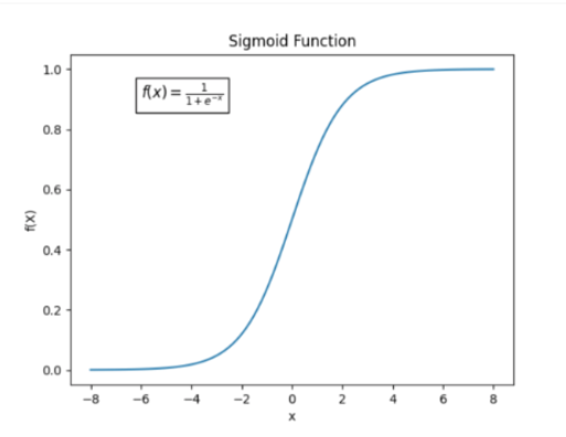
[!tip] During training, we want this model to generate high rewards for chosen answers and low rewards for rejected answers.
Similar to the Bradley-Terry parameterization form:
$$ Loss = -\log \sigma(r(x, y_w) - r(x, y_l)) $$
represents Chosen, represents the opposite. Therefore, when the model gives a high reward for chosen,
Thus the loss will be low, while if the model gives a low reward for the chosen answer, the loss will be very high.
The RewardTrainer class in HuggingFace accepts an AutoModelForSequenceClassification input (which is the model structure mentioned above).

Actor & Critic Model
Trajectories
As mentioned earlier, the core goal of Reinforcement Learning (RL) is to find a strategy (policy, ) that guides the agent’s actions to obtain the maximum possible expected return.
Mathematically, we represent this as finding the optimal strategy that maximizes the objective function :
The expected return represents the average total return the agent is expected to accumulate over many possible lifecycles or episodes when following strategy .
Its calculation method involves considering all possible trajectories () and calculating the weighted average (or integral) of the total return of each trajectory multiplied by the probability of that trajectory occurring under strategy .
- denotes the Expected Value when the trajectory is generated according to strategy .
- is the total return (reward) obtained on a single trajectory .
- is the probability that a specific trajectory occurs when the agent uses strategy .
A trajectory is a sequence of states and actions experienced by the agent, starting from an initial state. It is one possible “story” or “path” of the agent’s interaction with the environment.
- : State at time step .
- : Action taken at time step (usually based on state and strategy ).
We typically model the environment as stochastic. This means that executing the same action in the same state does not always lead to the exactly same next state . Randomness is involved.
The next state is drawn from a probability distribution conditioned on the current state and the action taken :
Considering stochastic state transitions and the Agent’s strategy, we can calculate the probability of the entire trajectory occurrence. It is obtained by multiplying the following terms:
- Probability of the Agent being in the initial state : .
- For each time step in the trajectory:
- Probability of the environment transitioning to state given and : .
- Probability of the agent selecting action in state according to its strategy: .
(Where is the length of the trajectory).
When calculating the total return of a trajectory, we almost always use discounted rewards. This means that rewards received earlier are more valuable than rewards received later.
Why?
- Reflects real-world scenarios (a dollar today is worth more than a dollar tomorrow).
- Avoids infinite return problems in continuous tasks (tasks without a fixed endpoint).
- Provides mathematical convenience.
We introduce a discount factor , where . The closer is to 0, the more “short-sighted” the Agent is (caring more about immediate benefits); the closer is to 1, the more “far-sighted” the Agent is (caring more about long-term returns).
The total discounted return of a trajectory is calculated as follows:
- is the immediate reward received at time step .
- is the discount coefficient applied to the reward at time step .
So what is a trajectory in LLM? As mentioned earlier, the model is the policy, the prompt is the state, and the next token is the action, so these s, a sequences in autoregressive generation make up the trajectory.

Policy Gradient
We have defined the goal of reinforcement learning: find an optimal strategy to maximize the expected return . Great. But how do we actually represent and find this strategy?
Usually, especially when dealing with complex problems, we don’t search through all possible strategies. We define a parameterized policy, denoted as . You can think of as a set of “knobs” or parameters—if our strategy is a neural network, then would be the weights and biases of the network.
Our goal now becomes: how to adjust these knobs to maximize our expected return?
[!note] Under strategy with parameter , the expected return of all possible trajectories:
This means the expected return depends on the trajectory , and the distribution of trajectories depends on the actions selected by our specific strategy . Changing changes the strategy, changes the trajectory, and thus changes the expected return.
[!note] We want to maximize by changing . In deep learning, gradient descent is generally used to minimize a loss function. Here, we want to maximize a function . So, we use gradient ascent conversely! It’s like climbing a hill—finding the steepest upward direction (i.e., gradient) and taking a step in that direction.
Our strategy is a neural network, and we will iteratively adjust its parameters to increase . This update rule will look very familiar (just replacing the minus sign in gradient descent with a plus sign):
- : Parameters at the -th iteration.
- : Learning rate (step size).
- : The gradient of expected return with respect to parameters , calculated at current parameters . It tells us which direction in the parameter space can maximize .

[!important] PG Derivation I’ll be a bit verbose at the beginning to re-introduce all the notations, ADHD-friendly derivation…
Step 1, reiterate that the object we are requesting the gradient for is the expected return :
$ \nabla{\theta} J(\pi{\theta}) = \nabla{\theta} E{\tau \sim \pi_{\theta}} [R(\tau)] $
Here:
- is the expected return.
- denotes the expected value, calculated over all possible trajectories (). Trajectory is a series of states and actions generated by the interaction between the Agent and the environment .
- indicates that these trajectories are generated according to our current strategy .
- refers to the total return (usually discounted return) obtained by a complete trajectory .
- is the gradient operator, indicating we need to find the partial derivative with respect to parameter .
Step 2, let’s expand the expression of expectation: What is the definition of expected value? For a random variable , its expectation can be calculated through its probability distribution :
- If it is a continuous variable:
- If it is a discrete variable:
In our example, the random variable is the trajectory return , and the probability distribution is the probability of trajectory occurrence (probability of trajectory occurring given strategy ). So, the expectation can be written in the form of an integral (or summation):
$ E{\tau \sim \pi{\theta}} [R(\tau)] = \int P(\tau|\pi_{\theta}) R(\tau) d\tau $
(Here the integral symbol is used to represent summing or integrating over all possible trajectories, which is more general). Substitute this into the formula in Step 1:
$ \nabla{\theta} J(\pi{\theta}) = \nabla{\theta} \int P(\tau|\pi{\theta}) R(\tau) d\tau $
Step 3: Move the gradient operator inside the integral sign
$ \nabla{\theta} \int P(\tau|\pi{\theta}) R(\tau) d\tau = \int \nabla{\theta} [P(\tau|\pi{\theta}) R(\tau)] d\tau $
Here requires a bit of calculus knowledge: under certain conditions (usually assumed to be met in reinforcement learning), we can exchange the order of differentiation and integration. Just like . Next, notice that is the total return of a determined trajectory, its value itself does not directly depend on the strategy parameter . (It is the strategy that influences which trajectory will happen, not what its return value is once this trajectory happens). So, the gradient only needs to act on :
$ = \int [\nabla{\theta} P(\tau|\pi{\theta})] R(\tau) d\tau $
This step tells us that the change in expected return is the effect of parameter changing causing the probability of each trajectory occurrence to change, multiplied by the return of that trajectory itself , and then accumulated over all trajectories.
Step 4: Log-derivative trick This is the most core and ingenious step in the entire derivation! We need to introduce an identity.
- Calculus Review (Chain Rule and Logarithmic Differentiation): Recall that the derivative of natural logarithm (usually refers to ) is .
- With a slight transformation, we get: 。 Now, we apply this trick to the gradient. Let correspond to , and independent variable correspond to parameter . Then:
Substitute this result into the integral in Step 3:
Step 5: Transform back to expectation form Observe the result from Step 4:
$ \int P(\tau|\pi{\theta}) [\nabla{\theta} \log P(\tau|\pi_{\theta}) R(\tau)] d\tau $
This conforms to the definition of expectation again! . Here, corresponds to everything inside the square brackets . So, the entire integral can be written back in the form of expectation:
$ = E{\tau \sim \pi{\theta}} [\nabla{\theta} \log P(\tau|\pi{\theta}) R(\tau)] $
Significant Meaning! We successfully converted the gradient of expectation into the expectation of a certain quantity (gradient times return) . This form is very important because it can be approximated by sampling! We don’t need to actually calculate the integrals of all trajectories. We just need to sample many trajectories , calculate the value in the brackets for each trajectory, and then average them to get an approximation of the gradient!
Step 6: Expression for grad-log-prob Now, we need to handle the term inside the expectation. Recall the trajectory (assuming trajectory length is T+1 states and T+1 actions, or T time steps). The probability of a trajectory occurring is:
$ P(\tau|\pi{\theta}) = p_0(s_0) \prod{t=0}^{T} P(s{t+1}|s_t, a_t) \pi{\theta}(a_t|s_t) $
: Probability of initial state .
: Environment Dynamics, probability of transitioning to state after executing action in state .
: Policy, probability of selecting action in state (this part depends on ).
Math Review (Logarithmic Properties): and . Take the logarithm of :
Now calculate the gradient of the above formula with respect to :
Math Review (Gradient Properties): Addition rule for gradients . Gradient only affects terms dependent on .
Key Points:
- Initial state probability typically does not depend on policy parameter , so .
- Environment dynamics describes the properties of the environment itself and also does not depend on policy parameter , so .
- Only policy depends on . So, the above formula simplifies to:
The gradient of the log probability of the entire trajectory equals the sum of the log probability gradients of each action step in that trajectory! This greatly simplifies the calculation.
Step 7: The Final Policy Gradient Theorem Substitute the simplified result from Step 6 back into the expectation formula in Step 5:
This is the final form (or one common form) of the Policy Gradient Theorem. The gradient of expected return with respect to parameter is equal to the expectation (average) over all possible trajectories of “sampling a trajectory , calculating the total return of that trajectory, and then multiplying it by the sum of policy log probability gradients corresponding to all (state, action) pairs in that trajectory”.
Obviously, obtaining all trajectories is extremely costly, for example, we want to sample all generated results of max_token_length=100, so we can use sample mean to approximate expectation:
[!note] Monte Carlo Approximation: * Run current strategy , collect trajectories, form dataset (let ).
- Approximate expectation value with the average of these samples:
Application to LM Policy
Through the generation process shown in the figure, we obtain the log probability of each state action pair in this sampled trajectory, and now we can backpropagate to calculate the gradient.

Then multiply each gradient by the reward from RM fed into the expression to run gradient ascent optimization:

High Variance
PG algorithms work well for small problems, but have some issues applied to language modeling.
[!note] The central limit theorem tells us: as long as the sample is large enough, the sample mean will be normally distributed, which allows us to better predict and analyze data. When the sample size is small, the fluctuation of sample mean will be large; even if the mean tends to normal distribution, the result of a single sampling may vary greatly. And we know that the cost of sampling many trajectories from LM is very high, which leads to the high variance problem of the estimator.
How to reduce variance without increasing sample size?
- Remove historical rewards: reward-to-go First, we must admit that the current action cannot affect the rewards already obtained in the past, and past rewards add unnecessary noise, which should be somewhat related to the credit assignment problem in RL. Therefore, removing past terms can avoid adding noise, bringing the estimated gradient closer to the true gradient. So instead of calculating trajectory rewards from scratch, we can only consider rewards for actions starting from the current time step.

- Introduce baseline RL research has confirmed that introducing a term dependent on state (such as a function calculating trajectory rewards, or a constant) can reduce variance. Here we choose Value Function .
Value Function
tells you what the expected reward for the remaining trajectory is based on the current strategy.
Examples of value definitions in classic RL scenarios and LM scenarios:

In practice, we use the LM we are trying to optimize for initialization, adding a linear layer on top of it to estimate value, so that the parameters of Transformer layers can be used for both language modeling (using the layer projecting tokens to vocabulary) and value estimation.

The reward-to-go mentioned earlier is called Q function in RL, which means the expected reward of starting from the current state, taking this action, getting immediate reward, and completing subsequent actions according to the strategy:

Then by introducing Value function, we get the difference between Q and V, and this difference is called Advantage function.

This advantage term represents how much better this specific action is relative to the average action that can be taken in state .

In the figure, the advantage function for moving downward from the state pointed by the red arrow will be higher than the advantage functions of other actions.
After multiplying the gradient by the advantage function, the effect becomes increasing the logprob of actions with high advantage for the strategy, and decreasing the log prob of actions bringing low average return.
[!note] In traditional reinforcement learning methods, Q Network and V Network are usually independent. That is, the Q function is used to estimate the total expected return of executing action in state , while V function only estimates the value of state . This requires two different neural networks to calculate these two values respectively.
However, now we introduce the advantage function , calculated based on the difference between Q value and V value, i.e.:
By expressing as the difference between and , we find that we only need to train one network to output , and then calculate Q value through reward and discount factor .
Therefore, only one neural network is needed, primarily to predict . The Q value is calculated by the following formula:
The advantage function is further calculated as:
Advantage Sampling
Short-step advantage estimators have large bias but small variance, while long-step advantage estimators have small bias but large variance. This trade-off is a part of reinforcement learning that needs careful selection and adjustment, depending on model stability requirements and training efficiency.
An example: “A person with short-term memory only remembers what happened yesterday. Although not comprehensive, it is stable; a person with long-term memory can see the full picture of the next few days, but may be interfered with by more unknown factors.”

GAE
To solve this bias-variance problem, GAE (Generalized Advantage Estimation) can be used, which is essentially a weighted sum of all advantage terms, with each term multiplied by a decay factor.
[!note] Now let’s talk about TD error Online learning has a beauty: you don’t need to wait until the end to update the strategy. So, Temporal Difference Error (TD Error) comes into play:
The key here is: TD error is actually an online estimation of the advantage function. It tells you whether your action at this moment makes the future state better than you expected. This error directly reflects the concept of advantage:
- If : “Hey, this action is better than I thought!” (Positive advantage).
- If : “Well, I thought it would be better…” (Negative advantage).
This allows you to adjust step by step your strategy without waiting for a whole episode to end to make changes. This is simply an excellent strategy for improving efficiency.
The purpose of GAE is to provide an estimate of advantage function that is better than original return or simple TD error in policy gradient algorithms, reducing gradient estimation variance and improving learning stability and efficiency.
This formula recursively defines generalized advantage estimation . It doesn’t just look at one-step TD error , but synthesizes TD error information from multiple future steps.
This recursive formula calculates backwards from the end of the trajectory (episode) (assuming is the last step, ):
- …
- General form: (assuming infinite step length or is 0 after termination state)
Parameter () is the key to GAE, controlling the bias and variance of estimation :
- When :
- . GAE degenerates into simple one-step TD error. This estimation has lower variance (because it only depends on the next step information), but may have higher bias (because it heavily relies on the possibly inaccurate estimate of ).
- When :
- . Through derivation, it can be proven that this is equivalent to , which is Monte Carlo return minus baseline. This estimate has lower bias (because it uses the complete actual return starting from time ), but variance is usually very high (because it accumulates randomness from multiple time steps).
- When :
- GAE interpolates between the above two extreme cases. The closer is to 0, the more biased it is towards low variance high bias TD estimation; the closer is to 1, the more biased it is towards high variance low bias MC estimation.
- By choosing appropriate (e.g., 0.97), GAE attempts to achieve a good balance between bias and variance, thereby obtaining an advantage estimate that is relatively accurate (controllable bias) and relatively stable (small variance).
Advantage of Language Models
As shown in the figure, the goal is to increase the logprob of token “Shanghai” in the current state and decrease the logprob of “chocolate”, because the advantage of choosing “Shanghai” is higher than the advantage of choosing “chocolate” (gibberish token).

Importance Sampling and Offline Learning
In many cases, we may want to calculate , but:
- It is difficult or impossible for us to directly sample from the target distribution .
- Or sampling from is inefficient. This is the problem in language models, where LM sampling cost is too high.
However, we might be able to easily sample from another alternative, or Proposal distribution .
Importance Sampling (IS) is a technique for estimating expectations of a target distribution by sampling from different distributions, converting an expected value calculated under probability distribution into an expected value of a related function calculated under a different probability distribution .
The key here is introducing importance weight . The function of this weight is bias correction: for a sample drawn from , if it has a higher probability of appearing in the target distribution (), give it a weight greater than 1; conversely, if it has a lower probability of appearing in (), give it a weight less than 1. Weighted averaging in this way yields an (usually unbiased or consistent) estimate of the original expectation .
Importance sampling allows us to:
- Draw samples from an easily sampled distribution .
- Estimate original expected value by calculating weighted average:
Back to our scenario. Previously we obtained On-Policy Policy Gradient Estimation:
[!info] Meaning of On-Policy: The strategy used to collect data and the strategy used for training are the same. Since calculation requires trajectories generated by sampling from current strategy . This means that after each strategy update, old data cannot be used directly, resulting in low sample efficiency. As for when mini_batch_num > 1, is the data used for subsequent updates still On-Policy? Strictly speaking, it feels like it’s not, so it can also be understood as Semi-On-Policy? (Expression implies not necessarily rigorous).
And On-Policy emphasizes whether the current strategy model can interact with the environment.
We hope to use data generated by old strategy in the past (these data may exist in large quantities) to estimate the gradient of current new strategy . This allows reusing data and improving sample efficiency.
Recall the principle of Importance Sampling IS: . Corresponding to our PG (simplifying to consider single-step decision):
- Target distribution corresponds to new strategy .
- Sampling distribution corresponds to old strategy .
- Importance weight is .
Applying importance weights to each term (each time step ) of On-Policy gradient yields standard Off-Policy estimation:
Now we have found a way to perform complete gradient ascent optimization without sampling from the strategy we are optimizing (model to be trained) every time, but sampling only once, saving the trajectory to memory/database, optimizing policy with mini-batch, and then initializing offline policy (sampled policy) with new policy.
PPO Loss
PPO Loss mainly consists of three parts: Policy Loss (), Value Function Loss (), and Entropy Bonus ().
1. Policy Loss ()
Clipped Surrogate Objective
This is the core of PPO. You will notice it looks a bit like the off-policy strategy gradient objective we derived using importance sampling earlier, but with a key modification.
: This is the importance sampling ratio, let’s call it . It is the probability of taking action in state according to current (online) strategy , divided by the probability of taking that action according to old (offline) strategy used when collecting trajectory data. This ratio corrects for the fact that data comes from a strategy slightly different from the one we are currently trying to improve.
: This is the advantage function estimate, calculated using GAE, which helps balance bias and variance. It tells us how much better or worse taking action in state is compared to taking the average action in that state (judged by current value function).
clipfunction: This is where the key point of PPO lies. It basically says: if probability ratio deviates too far from 1 (too high or too low), we “clip” it. So, if tries to become and is , it will be clipped to . If it tries to become , it will be clipped to . Parameter (epsilon) is a small hyperparameter (e.g. 0.1 or 0.2) that defines clipping range .minfunction: This objective function takes the smaller of the following two terms:Unclipped objective:
Clipped objective:
Why do this? The goal of policy gradient is to increase probability of actions with positive advantage and decrease probability of actions with negative advantage. However, when using importance sampling, if becomes very large, it may lead to huge updates and instability. PPO tries to keep the new strategy close to the old strategy by clipping this ratio.
- If (good action): We want to increase . The
minfunction means if grows beyond , the objective function will be limited to . This prevents the strategy from changing too much in a single update, even if the unclipped objective would suggest a larger increase. - If (bad action): We want to decrease . If shrinks below , the objective function will be limited to . (Note: When , the term is larger (closer to zero or positive) when is smaller, and is also larger when is smaller. Here
minactually means when ratio exceeds clipping boundary, we take the more pessimistic update step, or step that causes smaller change in log probability.) More precisely, when , the product will become more negative as increases. Theminoperation ensures that if deviates from interval, we won’t let the objective become too negative (that is, we won’t excessively lower the probability of that action).
2. Value Function Loss ()
This is exactly the same as before:
- is the output of the value network (i.e. adding a linear layer on top of LLM to predict expected cumulative reward starting from state ).
- The term (let’s call it or target value) is the actual sum of discounted rewards observed starting from state and following current strategy until end of episode. This is the empirical target we set for .
- This loss function is the Mean Squared Error (MSE) between predicted value and observed target value . We want the value function to accurately predict future rewards. This value function is crucial for calculating advantage .
3. Entropy Bonus ()
- Here (or more accurately , for all possible actions given state ) represents the action probability distribution output by current strategy in given state.
- The term is the entropy of this probability distribution. Entropy measures randomness or uncertainty of distribution. Uniform distribution (very random) has high entropy, while peaked distribution (very certain about an action) has low entropy.
- The loss term is negative entropy. When we minimize this in total loss (assuming is positive), we are actually maximizing the entropy of the strategy.
Encouraging higher entropy can promote exploration, making the strategy a bit more random, trying different actions (trying different tokens in LLM case), instead of converging too quickly to a possibly suboptimal deterministic strategy. This helps Agent discover better strategies.
Final Form
The final PPO loss is the weighted sum of these three parts:
- : Value function loss, weighted by . A common value for is around .
- : Entropy bonus (if , actually penalty for low entropy), weighted by . is usually a small positive constant (e.g. ), used to encourage exploration while not overwhelming the main policy objective.
Agent parameters (i.e. LLM weights) are updated by calculating the gradient of this combined loss and performing gradient descent.
Reference Model
Reward Hacking
A major problem in RL is reward-hacking, where the model might learn to always output tokens or sequences that bring good rewards but make no sense to humans, such as saying “thank you” ten times in a row to boost politeness score. So we hope the aligned model’s (after RL post-training) output is as close as possible to the original model’s output.
Therefore, there will be another model with frozen weights (ref model). When the model we want to optimize generates rewards through reward model in each step of each trajectory, this reward will subtract the KL divergence between log prob of ref model and optimized model as a penalty term to prevent the model from generating answers that differ too much from the original model, thus preventing the cheating phenomenon mentioned above.

Code walk through
trl
class AutoModelForCausalLMWithValueHead(PreTrainedModelWrapper):
# ... (class attributes like transformers_parent_class) ...The core purpose of this class is to bundle a standard Causal Language Model (Causal LM) (our Actor Model, strategy responsible for generating text) with a Value Head (our Critic Model, responsible for estimating state value V(s)). In PPO / Actor Critic algorithms, we need both strategy and value function, and this class provides a unified model structure to output both simultaneously.
def __init__(self, pretrained_model, **kwargs):
super().__init__(pretrained_model, **kwargs) # Basic settings
v_head_kwargs, _, _ = self._split_kwargs(kwargs) # Separate args for ValueHead
# Ensure input uses a model with language model output capability
if not any(hasattr(self.pretrained_model, attribute) for attribute in self.lm_head_namings):
raise ValueError("The model does not have a language model head...")
# Create ValueHead instance, which will learn to predict state value V(s)
self.v_head = ValueHead(self.pretrained_model.config, **v_head_kwargs)
# Initialize ValueHead weights
self._init_weights(**v_head_kwargs) # Default random init, can also specify normal distribution init- Acting as Actor: That is our language model
pretrained_model, which generates responses (action a, i.e., a series of tokens) based on current prompt (state s). - Critic: Evaluate “good/bad” of Actor in a certain state s, i.e., output . This is the task of linear layer
self.v_head.
def forward(
self,
input_ids=None, # Input token IDs (state s)
attention_mask=None,
past_key_values=None, # For speeding up generation
**kwargs,
):
# Force underlying model to output hidden_states, ValueHead needs them as input
kwargs["output_hidden_states"] = True
# ... (some details of processing past_key_values and PEFT, can be ignored in core PPO understanding)
# 1. Actor (Base Language Model) calculation
base_model_output = self.pretrained_model(
input_ids=input_ids,
attention_mask=attention_mask,
**kwargs,
)
# 2. Extract Actor output (for policy update) and Critic input
lm_logits = base_model_output.logits # Actor output: probability distribution predicting next token
# This is the basis for calculating L_POLICY and L_ENTROPY in PPO
last_hidden_state = base_model_output.hidden_states[-1] # Critic input: hidden state of last layer of LM,
# Represents the representation of current state s
# (Optional) Language model's own loss, usually not directly used in RL stage
loss = base_model_output.loss
# (Ensure data and model are on same device)
if last_hidden_state.device != self.v_head.summary.weight.device:
last_hidden_state = last_hidden_state.to(self.v_head.summary.weight.device)
# 3. Critic (ValueHead) calculation
# ValueHead receives state representation, outputs value estimation V(s) for that state
value = self.v_head(last_hidden_state).squeeze(-1) # This is the basis for calculating value loss L_VF and advantage A_hat in PPO
# (Ensure logits are float32 for numerical stability)
if lm_logits.dtype != torch.float32:
lm_logits = lm_logits.float()
# Return Actor's logits, LM loss (may be None), and Critic's value
return (lm_logits, loss, value)For every step of PPO-RLHF training:
- We input a batch of current prompts (sequence
input_ids) into the model. self.pretrained_model(Actor) will calculate (Rollout)lm_logits. These logits represent the probability distribution of which tokens the model thinks should be generated next given the current prompt. PPO’s policy loss and entropy bonus both need to be calculated based on this probability distribution .- At the same time, we take
last_hidden_statefrombase_model_output. This can be seen as a vector representation of current prompt (state s). - This
last_hidden_stateis sent intoself.v_head(Critic), outputting a scalarvalue. Thisvalueis the model’s value estimate for current state s. PPO’s value function loss is to optimize this to be as close as possible to true return. And this is also a key component for calculating advantage function , which in turn guides the calculation of . - The same prompt + response sequence is input to Reward and Reference model for inference to get reward and log probs (calculating KL penalty).
So with one forward call, we simultaneously obtain core information needed to update Actor (Strategy) and Critic (Value Function).
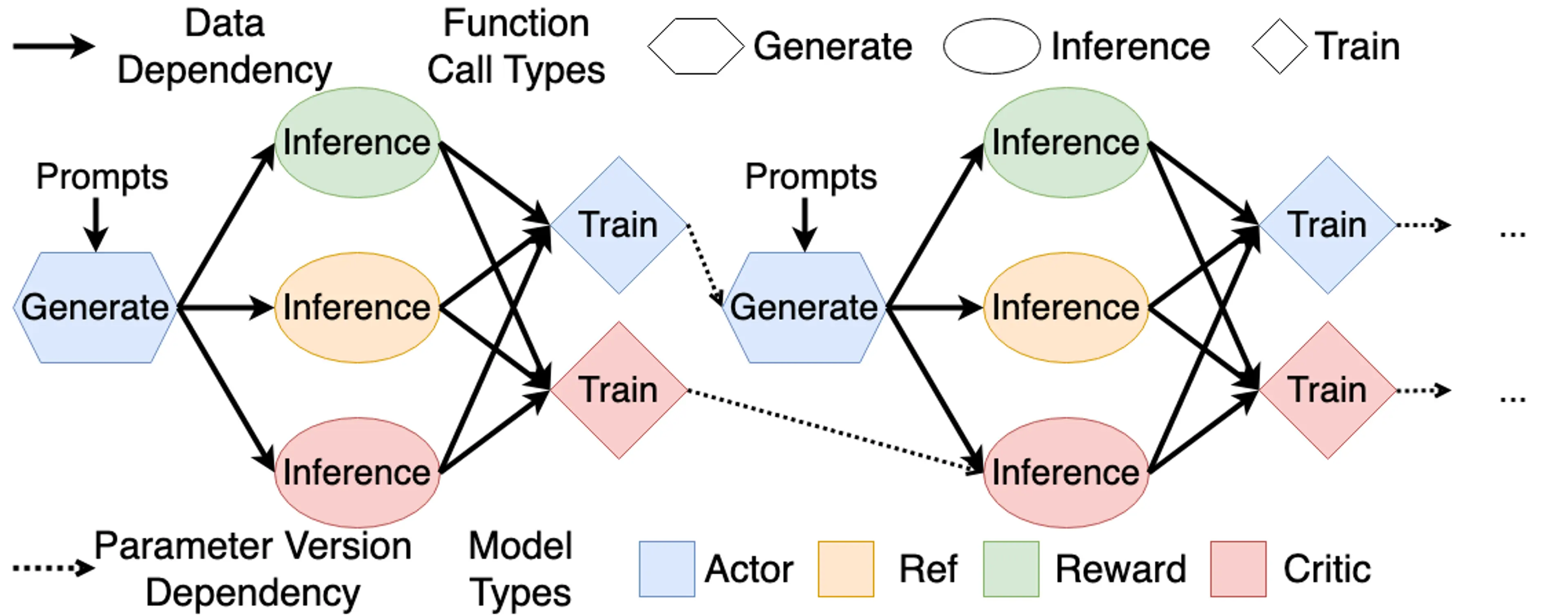
The training flow can be understood with the help of the following diagram:

[!tip] In RLHF, only Actor needs Prefill + Decode (Complete Auto-Regressive Generation) during experience collection (Rollout), other models only process existing responses to get logprob and value etc., doing only Prefill.
In addition, Actor involves training and inference (referring to Rollout), so it requires training engine (such as Megatron, DeepSpeed and FSDP) + rollout engine (such as SGLang and vLLM) to complete their tasks respectively; Critic reuses internal representations in forward during training for new value prediction during inference, so it runs in same training engine; while Reference and Reward model both only use inference engine to get logprob and reward.
verl
Along with OpenRLHF etc., are excellent RLHF frameworks, a good introductory guide: [AI Infra] VeRL Framework Introduction & Code Walkthrough