Introduction to Policy Gradient

This article is a record of learning from Andrej Karpathy’s Deep RL Bootcamp and his blog post: Deep Reinforcement Learning: Pong from Pixels.

Progress in RL isn’t primarily driven by novel, stunning ideas:

AlexNet in 2012 was mostly an extension (deeper, wider) of 1990s ConvNets. The 2013 paper on Deep Q-Learning for ATARI games was an implementation of a standard algorithm (Q-Learning with function approximation, Sutton 1998) where the function approximator happened to be a ConvNet. AlphaGo used policy gradients combined with Monte Carlo Tree Search (MCTS), which are also standard components. Of course, making these algorithms work effectively requires immense skill and patience, and many clever improvements were developed on top of old algorithms, but roughly speaking, the main driver of recent progress isn’t the algorithms themselves but (similar to computer vision) computing power, data, and infrastructure. ——Andrej Karpathy

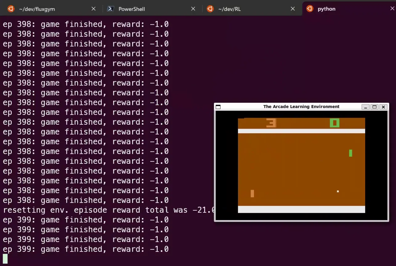
ATARI Pong

Pong is a special case of a Markov Decision Process (MDP): a graph where each node represents a specific game state and each edge represents a possible (often stochastic) transition. Each edge is also assigned a reward, and the goal is to calculate how to take optimal actions in any state to maximize rewards.

Game Principles

We receive image frames (byte arrays representing pixel values 0-255) and must decide whether to move the paddle UP or DOWN (binary choice). After choosing, the game simulator executes the action and provides a reward: +1 if the ball passes the opponent (winning a point), -1 if we miss, and 0 otherwise. Our goal is to move the paddle to maximize total rewards.

In exploring solutions, we’ll minimize assumptions about the game, treating it as a toy case for learning.

Policy Gradient

Policy Gradient algorithms are favored for their end-to-end nature: they have an explicit policy and a principled method for directly optimizing expected rewards.

Policy Network

We define an Agent’s policy network that takes the game state and decides the action (UP or DOWN). We’ll use a two-layer NN that takes raw pixels ($210 \times 160 \times 3 = 100,800$) and outputs a single number representing the probability of moving UP. We typically use a stochastic policy rather than deterministic decisions, sampling from the distribution (tossing a biased coin with probability $p$ and $1-p$) to obtain the actual move. This allows the agent to sometimes choose sub-optimal actions, potentially discovering better strategies.

h = np.dot(W1, x)     # Compute hidden layer activations (dot product of weights and input)
h[h < 0] = 0          # ReLU: set values < 0 to 0, i.e., max(0, h)
logp = np.dot(W2, h)  # Compute log probability of moving UP, W2 is hidden-to-output weights
# Convert log probability to a probability value (0, 1) using Sigmoid
p = 1.0 / (1.0 + np.exp(-logp))  

Intuitively, neurons in the hidden layer (weights along rows of W1) can detect various game scenarios, while weights in W2 decide whether to move UP or DOWN in each case. Initially, random parameters result in the player twitching in place; the goal is to find W1 and W2 that master the game.

Preprocessing

Ideally, we want to feed at least 2 frames into the network to detect motion. To simplify, we can preprocess the input as the difference between the current and previous frames.

Credit Assignment Problem

Non-zero rewards might only appear after hundreds of timesteps. We don’t know which specific action—the last one, frame 10, or frame 90—or which parameters were responsible.

This is the Credit Assignment Problem (CAP) in RL. In our case, we get a +1 reward because we happened to bounce the ball into a good trajectory past the opponent’s paddle, but that action happened many frames before the reward. Many actions taken after that point may not have contributed to the reward at all.

Supervised Learning

Before diving into the policy gradient solution, let’s revisit Supervised Learning (SL). SL aims to adjust parameters via backpropagation so the model increasingly predicts the correct label.

The model takes an image and outputs probabilities. For example, log probabilities for UP and DOWN might be $(-1.2, -0.36)$, corresponding to 30% and 70%. If we know the correct label (e.g., UP), our goal is to maximize its log probability. We compute the gradient of $\log p(y=UP \mid x)$ and use backpropagation to adjust parameters.

• If a parameter’s gradient is -2.1, decreasing it (e.g., by 0.001) increases the log probability by $2.1 \times 0.001$.
• After the update, the network will be slightly more likely to predict UP in similar situations.

Policy Gradient

In RL, we have no “correct” labels. This is where PG comes in:

• Initial Phase: The model computes probabilities (e.g., 30% UP, 70% DOWN). We randomly sample an action, say DOWN, and execute it.
• Gradient Calculation: Like SL, we can immediately compute the gradient of the log probability for the chosen action (DOWN). But we don’t know yet if it was a good move.
• Await Feedback: We wait until the game ends to get a reward. In Pong, if we lose, we get -1. We use this -1 as a weight for the DOWN action gradient during backpropagation.
• Optimization: Since DOWN led to a loss, the gradient update makes the network less likely to choose DOWN in the future.

Thus, PG adjusts the policy based on delayed rewards, favoring actions that lead to success.

Training Protocol

The full training flow is:

1. Initialize the policy network with random W1 and W2.
2. Play 100 Pong games (rollouts).

Suppose each game has 200 frames, totaling 20,000 UP/DOWN decisions. We compute gradients for each decision, telling us how to nudge parameters to favor those decisions.

3. Update:

• If we won 12 games, the 2,400 decisions in those games get a positive update (gradient weight +1.0), encouraging them.
• Since we lost 88 games, the 17,600 decisions in those games get a negative update, discouraging them.

The network slightly increases the probability of effective actions and slightly decreases that of ineffective ones.

4. Repeat steps 2 and 3 using the improved policy, continuously optimizing.

[!Karpathy’s summary] Policy Gradients: Run a policy for a while. See what actions led to high rewards. Increase their probability.

Each circle is a state, each arrow a transition with a sampled action. With PG, we take winning episodes and slightly encourage every action within them, and vice versa for losing ones.

Question: If we made a correct “bounce ball” decision at frame 50 but eventually lost at frame 150, every action in that episode is discouraged. Will this hurt our frame 50 decision?

Yes, it will. However, across thousands or millions of games, correct decisions will lead to wins more often. On average, the final policy will learn the correct actions.

Link Between Policy Gradient and Supervised Learning

Policy Gradient is similar to SL, except:

1. We use model-sampled actions as “labels.”
2. We weight the loss function based on the outcome (reward/punishment).

In standard SL, the goal is to maximize $\log p(y_i \mid x_i)$ for each sample.

In RL, we lack correct labels $y_i$. So we treat sampled actions as “fake labels” and adjust loss weights for each sample based on the final outcome (win/loss) to favor successful actions.

The RL loss function looks like $\sum_i A_i \log p(y_i \mid x_i)$ where:

• $y_i$ is the sampled action (“fake label”).
• $A_i$ is the advantage, measuring the outcome.
  • $A_i = 1.0$ for a win.
  • $A_i = -1.0$ for a loss.

RL can be seen as SL on a shifting dataset (episodes) sampled from games, with loss weights adjusted by results.

General Advantage Function

Previously, we judged actions by the win/loss of an entire game. In general RL, we get immediate rewards $r_t$ at each step.

Discounted Reward

A common approach is using Discounted Reward to calculate the cumulative return following an action:

• $\gamma$ is the discount factor (e.g., 0.99), reducing the weight of future rewards.
• Rewards further in the future are diminished more.

Normalize Returns

After computing $R_t$ for all actions (e.g., 20,000 actions in 100 Pong games), it’s standard to normalize them by subtracting the mean and dividing by the standard deviation:

Normalization ensures roughly half the actions in a batch are encouraged and half discouraged. Mathematically, this controls the variance of the policy gradient estimate, leading to more stable updates and faster convergence.

PG Derivation

Policy Gradient is a special case of a general score function gradient estimator. Consider:

$E_{x\sim p(x|\theta)}[f(x)]$

Where:

• $f(x)$ is a scalar score function (reward or advantage).
• $p(x;\theta)$ is a probability distribution parameterized by $\theta$ (the policy network).

Goal: Adjust $\theta$ to increase the score of samples.

[!Derivative of log trick] Basic property:

So:

[!OpenAI Spinning Up Version:]

This is an expectation, estimable via sample means. Given trajectories $\mathcal{D} = \{\tau_i\}_{i=1,...,N}$ collected under policy $\pi_{\theta}$, the gradient is estimated as: ${g} = \frac{1}{|\mathcal{D}|} \sum_{\tau \in \mathcal{D}} \sum_{t=0}^{T} \nabla_{\theta} \log \pi_{\theta}(a_t |s_t) R(\tau)$ where $|\mathcal{D}|$ is the number of trajectories. This computable expression allows us to update the policy using sampled experience.

Practice in GYM

Model Initialization

H = 200 # Neurons in hidden layer
batch_size = 10 # Update every N episodes
learning_rate = 1e-4
gamma = 0.99 # Discount factor
 
# Model initialization
D = 80 * 80 # Input: 80x80 grid
model = {}
model['W1'] = np.random.randn(H,D) / np.sqrt(D) # "Xavier" initialization
model['W2'] = np.random.randn(H) / np.sqrt(H)

Utility Functions

def prepro(I):
    """ Preprocess 210x160x3 uint8 frame into 6400 (80x80) 1D float vector """
    I = I[35:195] # crop
    I = I[::2,::2,0] # downsample
    I[I == 144] = 0 # erase background
    I[I == 109] = 0 # erase background
    I[I != 0] = 1 # everything else (paddles, ball) to 1
    return I.astype(np.float64).ravel()
 
def discount_rewards(r):
    """ Compute discounted rewards """
    discounted_r = np.zeros_like(r)
    running_add = 0
    for t in reversed(range(0, r.size)):
        if r[t] != 0: running_add = 0 # Reset sum for game boundary (Pong specific)
        running_add = running_add * gamma + r[t]
        discounted_r[t] = running_add
    return discounted_r

Policy Network

def policy_forward(x):
    h = np.dot(model['W1'], x)
    h[h<0] = 0 # ReLU
    logp = np.dot(model['W2'], h)
    p = sigmoid(logp)
    return p, h # Probability of action 2, and hidden state
 
def policy_backward(eph, epdlogp):
    """ Backpropagation """
    dW2 = np.dot(eph.T, epdlogp).ravel()
    dh = np.outer(epdlogp, model['W2'])
    dh[eph <= 0] = 0 # ReLU backprop
    dW1 = np.dot(dh.T, epx)
    return {'W1':dW1, 'W2':dW2}

Main Loop

while True:
    # Preprocess observation
    cur_x = prepro(observation)
    x = cur_x - prev_x if prev_x is not None else np.zeros(D)
    prev_x = cur_x
 
    # Forward pass and sample action
    aprob, h = policy_forward(x)
    action = 2 if np.random.uniform() < aprob else 3
 
    # Record history
    xs.append(x) # observation
    hs.append(h) # hidden state
    y = 1 if action == 2 else 0 # "fake label"
    dlogps.append(y - aprob) # gradient encouraging sampled action
 
    # Step environment
    observation, reward, done, info = env.step(action)
    reward_sum += reward
    drs.append(reward) # record reward

Episode End Handling

    if done:
        episode_number += 1
 
        # Stack history for this episode
        epx = np.vstack(xs)
        eph = np.vstack(hs)
        epdlogp = np.vstack(dlogps)
        epr = np.vstack(drs)
        xs,hs,dlogps,drs = [],[],[],[] # Reset buffers
 
        # Compute discounted and normalized rewards
        discounted_epr = discount_rewards(epr)
        discounted_epr -= np.mean(discounted_epr)
        discounted_epr /= np.std(discounted_epr)
 
        epdlogp *= discounted_epr # Scale gradient by advantage (Core of PG)
        grad = policy_backward(eph, epdlogp)
        for k in model: grad_buffer[k] += grad[k] # accumulate gradients over batch

Parameter Updates

    if episode_number % batch_size == 0:
        for k,v in model.items():
            g = grad_buffer[k]
            rmsprop_cache[k] = decay_rate * rmsprop_cache[k] + (1 - decay_rate) * g**2
            model[k] += learning_rate * g / (np.sqrt(rmsprop_cache[k]) + 1e-5)
            grad_buffer[k] = np.zeros_like(v) # reset buffer

Karpathy’s Reflection

For humans, we say “control a paddle to bounce the ball past the AI.” In standard RL, we assume an arbitrary reward function and learn via interaction. Humans bring massive prior knowledge (physics of ball trajectories, intuitive psychology of opponents) and require visual feedback. For PG, even if we randomly permuted every pixel in the frames, a fully connected policy network wouldn’t even notice the difference.

Thus, PG is a brute-force method that discovers correct actions and internalizes them into a policy.

PG can easily beat humans in many games—especially those requiring frequent rewards, precise control, fast reactions, and minimal long-term planning. Short-term action-reward correlations are easily “noticed” and refined. In Pong, late-stage agents wait until the ball is close, move rapidly to intercept, and fire it back with high vertical velocity. In many ATARI games (Pinball, Breakout), Deep Q-Learning similarly surpassed human baselines.