Reinforcement Learning Basics and Q-Learning

This year, I used the DeepSeek-Math-7B-RL model in a Kaggle competition and treated Claude 3.5 Sonnet as my teacher. The power of both models is inseparable from RL. I had a hunch that the technology in this field is both powerful and elegant, so I decided to dive in. Since my foundation wasn’t solid enough for OpenAI’s Spinning Up, I chose the Hugging Face DeepRL introductory course.

:::note{title=“Side Note”} Truth be told, after my college entrance exams, I chose AI because of my interest in “making AI understand the world through rewards and punishments, like playing a game.” Ironically, I didn’t actually touch RL until the summer of my junior year.

:::

Introduction

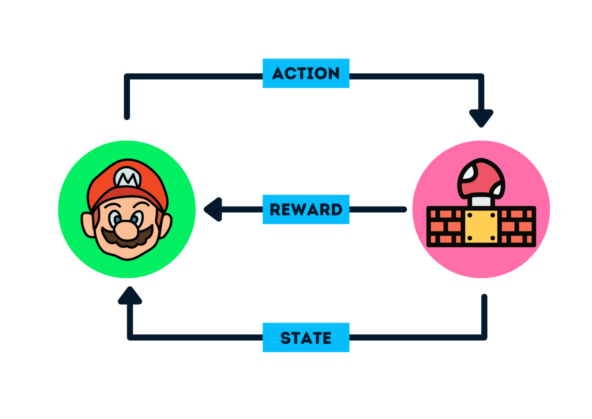
The core idea of Reinforcement Learning (RL) is that an agent (AI) learns from its environment by interacting with it (through trial and error) and receiving rewards (positive or negative) as feedback for its actions.

:::assert Formal Definition: Reinforcement Learning is a framework for solving control tasks (also called decision-making problems) by building agents that learn from an environment through trial and error, receiving rewards (positive or negative) as unique feedback. :::

Reinforcement Learning Cover

The Agent receives the first frame from the environment, state $S_0$ . Based on $S_0$ , the Agent takes action $A_0$ (e.g., move right). The environment transitions to a new frame (new state $S_1$ ) and gives the agent a reward $R_1$ (e.g., +1 for surviving).

The Agent’s goal is to maximize its cumulative rewards, known as the expected return.

The Reward Hypothesis: The Core Idea of RL

RL is based on the reward hypothesis, which states that all goals can be described as the maximization of expected return (expected cumulative reward). In RL, to achieve optimal behavior, we aim to learn to take actions that maximize expected cumulative rewards.

Two Types of Tasks

Episodic: Has a clear starting and ending point (e.g., a game level).
Continuous: Has a starting point but no predefined ending point (e.g., autonomous driving).

Difference Between State and Observation

State: A complete description of the world’s state (no hidden information), like a chessboard.
Observation: A partial description of the state, like a frame from a Mario game.

Policy-based Methods

In this method, the policy is learned directly. It maps each state to the best corresponding action or a probability distribution over the set of possible actions.

Value-based Methods

Instead of training a policy, we train a value function that maps each state to the expected value of being in that state. DQN training

The Exploration/Exploitation Trade-off

In RL, we must balance the degree of exploring the environment with exploiting known information.

Epsilon greedy strategy

Where Does “Deep” Come From?

Deep neural networks are introduced to solve reinforcement learning problems.

Q-learning results

Practical Example - HUGGY

I recommend playing with this in Colab. If running in WSL2, you’ll need a virtual display setup:

import os
os.environ['PYVIRTUALDISPLAY_DISPLAYFD'] = '0'
 
from pyvirtualdisplay import Display
display = Display(visible=0, size=(1400, 900))
display.start()

Deep Q-learning

State Space

We want to train Huggy to pick up a stick we throw. This means it needs to move toward the stick correctly.

Information we provide:

Target (stick) position.
Relative position between Huggy and the target.
Orientation of its legs.

Based on this, Huggy uses its Policy to decide the next action to achieve the goal.

Action Space

The actions Huggy can perform.

Frozen Lake environment

Joint motors drive Huggy’s legs.

To reach the goal, Huggy must learn how to correctly rotate each joint motor to move.

Reward Function

Our reward function:

Directional Reward: Reward for getting closer to the target.
Goal Achievement Reward: Reward for reaching the stick.
Time Penalty: A fixed penalty for each action, forcing it to reach the stick quickly.
Rotation Penalty: Penalty for excessive or overly fast rotations.

Introduction to Q-Learning

Value-based

v_{\pi}(s) = \mathbb{E}_{\pi} \left[ R_{t+1} + \gamma R_{t+2} + \gamma^2 R_{t+3} + \cdots \,|\, S_t = s \right]

Starting from state s, we act according to policy $\pi$ .
We accumulate future rewards, but distant rewards are diminished by the discount factor $\gamma$ .
The value function calculates the expected “return” for the entire future starting from the current state.

The goal of an RL agent is to have an optimal policy $\pi$ *.

Relationship Between Value and Policy

Finding the optimal value function yields the optimal policy.

\pi^*(s) = \arg \max_{a} Q^*(s, a)

$\pi^*(s)$ : The optimal policy, the best action to take in state $s$ .
$Q^*(s, a)$ : The state-action value function, representing the expected discounted future return when choosing action $a$ in state $s$ .
$\arg \max_{a}$ : Choosing action $a$ that maximizes $Q^*(s, a)$ .

If we have the optimal $Q^*(s, a)$ , the optimal policy $\pi^*(s)$ is simply choosing the action $a$ that maximizes future expected returns in each state $s$ .

Two Types of Value-Based Methods

Imagine a mouse in a maze looking for cheese:

State Value Function: The mouse’s emotional expectation at a specific position: “If I start from here and follow my policy, what’s my chance of finding cheese?”
Action Value Function: Goes further: “If I start here and choose to move right, what’s my probability of success?” This helps the mouse evaluate different actions in each state.

1. State Value Function

$V_\pi(s)$ evaluates the expected cumulative reward starting from state $s$ under policy $\pi$ . It measures “how good is it to be in this state if I follow my policy?”

V_\pi(s) = \mathbb{E}_\pi[G_t | S_t = s]

$V_\pi(s)$ : Value of state $s$ .
$G_t$ : Cumulative reward starting from time $t$ : $G_t = R_{t+1} + \gamma R_{t+2} + \gamma^2 R_{t+3} + \dots$
$\mathbb{E}_\pi[\cdot]$ : Expectation under policy $\pi$ .

DQN architecture

In the example above, each cell’s value is its state value. A value of $-6$ means the expected return from that cell is poor (far from cheese), while $-2$ is much better.

2. Action Value Function

$Q_\pi(s, a)$ evaluates the expected cumulative reward after taking action $a$ in state $s$ under policy $\pi$ .

Q_\pi(s, a) = \mathbb{E}_\pi[G_t | S_t = s, A_t = a]

$Q_\pi(s, a)$ : Value of the state-action pair $(s, a)$ .
Unlike the state value function, it assesses the long-term return of a specific action $a$ from state $s$ .

Target network

In the maze, if the mouse is in state $s$ and can move in four directions, $Q_\pi(s, a)$ tells it the expected return for each direction. Moving right might have a higher value than moving left if it leads closer to the cheese.

Summary of Differences

State Value Function $V_\pi(s)$ : Only considers the cumulative expected return from a state following a policy. It doesn’t care about the specific first action.
Action Value Function $Q_\pi(s, a)$ : More granular, considering the expected return after taking a specific action in that state.

Bellman Equation

Back to the mouse: if each step gives a reward of -1:

V(St) = (-1) + (-1) + (-1) + (-1) + (-1) + (-1) = -6

Cumulative return from $St$ to the end is -6.

V(St+1) = (-1) + (-1) + (-1) + (-1) + (-1) = -5

Calculating this directly for every path is expensive. The Bellman Equation provides a recursive shortcut.

Core idea: A state’s value is the immediate reward plus the discounted value of the next state.

V_\pi(s) = \mathbb{E}_\pi[R_{t+1} + \gamma V_\pi(S_{t+1}) | S_t = s]

If $\gamma = 1$ , $V(St+1) = -5$ , and $R_{t+1} = -1$ : Q-learning algorithm Which matches our direct calculation.

:::note{title=“Dynamic Programming”} The recursive nature of the Bellman Equation is similar to Dynamic Programming (DP), which breaks problems into smaller subproblems and stores solutions to avoid redundant calculations. :::

Role of the Discount Factor $\gamma$

Low $\gamma$ (e.g., 0.1): Focus on immediate rewards, ignoring the distant future.
$\gamma = 1$ : All future rewards are as important as current ones.
Extremely high $\gamma$ : Physically meaningless; future value is infinitely inflated.

Monte Carlo vs. Temporal Difference Learning

Both are strategies for training value or policy functions using experience.

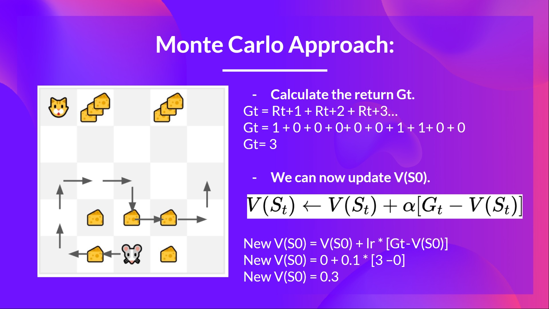
Monte Carlo: Learning at the End of an Episode

Monte Carlo (MC) estimates values by averaging full returns. We update the value function only after an episode ends, using the complete experience.

Record: State, action, reward, next state.
Calculate Total Return $G_t$ .
Update $V(s)$ : $V(S_t) \leftarrow V(S_t) + \alpha [G_t - V(S_t)]$ Where $\alpha$ is the learning rate.

Example:

Initial $V(S) = 0$ , $\alpha = 0.1$ , $\gamma = 1$ .
Mouse gets total return $G_0 = 3$ . $V(S_0) = 0 + 0.1 \times (3 - 0) = 0.3$

Temporal Difference (TD) Learning: Learning at Every Step

TD Learning updates after every step based on immediate reward $R_{t+1}$ and the estimated value of the next state $V(S_{t+1})$ .

V(S_t) \leftarrow V(S_t) + \alpha [R_{t+1} + \gamma V(S_{t+1}) - V(S_t)]

This is Bootstrapping: updating based on existing estimates ( $V(S_{t+1})$ ) rather than complete samples ( $G_t$ ).

Example:

Initial $V(S) = 0$ .
Mouse moves left, gets $R_{t+1} = 1$ .
TD Target: $TD_{Target} = R_{t+1} + \gamma V(S_{t+1}) = 1 + 1 \times 0 = 1$ .
Update: $V(S_0) = 0 + 0.1 \times (1 - 0) = 0.1$ .

Comparison: Bias vs. Variance

Monte Carlo: Waits for episode end. Uses actual $G_t$ .
- Unbiased: Estimates match real expected values.
- High Variance: Multi-step returns accumulate randomness.
- Great for global experience evaluation without a model.
TD Learning: Updates immediately. Uses estimated returns.
- Biased: Initial estimates are arbitrary. Bias decreases over time. Bias + off-policy + neural networks can lead to the “deadly triad” (instability).
- Low Variance: Only single-step randomness.
- Great for real-time updates.

Q-Learning Terminology

Q-Learning is an off-policy, value-based method using TD methods to train the Q-function. “Q” stands for Quality—the value of an action in a state.

DQN final results

Given state and action, Q outputs a Q-value.

Value vs. Reward: | Term | Explanation | | --- | --- | | Value | Expected cumulative reward (long-term). | | Reward | Immediate feedback for an action. |

Internally, the Q-function is encoded by a Q-Table—a “cheat sheet” of state-action pair values.

Experience replay

The optimal Q-Table defines the optimal policy:

\pi^*(s) = \arg \max_a Q^*(s, a)

Algorithm Workflow

Algorithm pseudocode:

SARSA vs Q-learning

Step 1: Initialize Q-Table

Usually initialized to 0. Cartpole environment

def initialize_q_table(state_space, action_space):
	Qtable = np.zeros((state_space, action_space))
	return Qtable

Step 2: Choose action via ε-greedy strategy

Balances exploration and exploitation by gradually decreasing exploration probability.

Probability $1 - \epsilon$ : Choose action with highest Q-value (exploitation).
Probability $\epsilon$ : Choose random action (exploration).

Q-table visualization

Early: $\epsilon = 1.0$ (pure exploration).
Later: $\epsilon$ decreases (exploitation increases).

Q-learning update rule

def greedy_policy(Qtable, state):
    return np.argmax(Qtable[state][:])
 
def epsilon_greedy_policy(Qtable, state, epsilon):
    if random.uniform(0,1) > epsilon:
        return greedy_policy(Qtable, state) # Exploit
    else:
        return env.action_space.sample() # Explore

Step 3: Execute $A_t$ , observe $R_{t+1}$ and $S_{t+1}$

The core step where feedback is received and the agent transitions.

Step 4: Update $Q(S_t, A_t)$

Using the TD update rule (bootstrapping):

Q(S_t, A_t) \leftarrow Q(S_t, A_t) + \alpha \left[ R_{t+1} + \gamma \max_a Q(S_{t+1}, a) - Q(S_t, A_t) \right]

Update is based on the best possible Q-value in the next state.

def train(n_training_episodes, min_epsilon, max_epsilon, decay_rate, env, max_steps, Qtable):
  for episode in tqdm(range(n_training_episodes)):
    epsilon = min_epsilon + (max_epsilon - min_epsilon)*np.exp(-decay_rate*episode)
    state, info = env.reset()
    for step in range(max_steps):
      action = epsilon_greedy_policy(Qtable, state, epsilon)
      new_state, reward, terminated, truncated, info = env.step(action)
      # Q-update:
      Qtable[state][action] = Qtable[state][action] + learning_rate * (reward + gamma * np.max(Qtable[new_state]) - Qtable[state][action])
      if terminated or truncated: break
      state = new_state
  return Qtable

Q-learning convergence

Off-policy vs. On-policy

On-policy: Learns the policy it is currently executing. (SARSA)
Off-policy: Learns a policy different from the one it is executing (e.g., learning the optimal policy while executing an exploratory one). (Q-Learning)

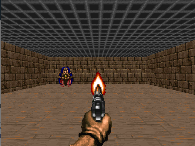
But for complex environments like Doom with millions of states, Q-Tables are impossible.

On-policy vs Off-policy

This is where Deep Q-Learning comes in, using a neural network to approximate Q-values.