banner
Nagi-ovo

Nagi-ovo

Breezing homepage: [nagi.fun](nagi.fun)
github

Implementing a minimalist automatic differentiation framework from scratch

Code repository: https://github.com/karpathy/nn-zero-to-hero

Andrej Karpathy is the author and main lecturer of the famous deep learning course Stanford CS 231n, and is also one of the founders of OpenAI. "micrograd" is a small, educational project he created. This project implements a very simplified automatic differentiation and gradient descent library, which requires learners to have only the most basic knowledge of calculus, for teaching and demonstration purposes.

Introduction to Micrograd#

Micrograd is essentially an autograd engine, and its real purpose is to implement backpropagation.

Backpropagation is an algorithm that efficiently computes the gradient of a certain loss function with respect to the weights in a neural network. This allows us to iteratively adjust the weights of the neural network to minimize the loss function, thereby improving the accuracy of the network. Thus, backpropagation becomes the mathematical core of any modern deep neural network library (such as PyTorch, JAX).

Types of operations supported by micrograd:

from micrograd.engine import Value

a = Value(-4.0)
b = Value(2.0)
c = a + b # The child nodes of C are A and B, because C maintains pointers to the value objects of A and B
d = a * b + b**3
c += c + 1
c += 1 + c + (-a)
d += d * 2 + (b + a).relu()
d += 3 * d + (b - a).relu()
e = c - d
f = e**2
g = f / 2.0
g += 10.0 / f # Output of the forward pass
print(f'{g.data:.4f}') # prints 24.7041, the outcome of this forward pass
g.backward() # Initialize backpropagation at node G, recursively referencing the chain rule from calculus to evaluate the derivative of G with respect to all internal nodes
print(f'{a.grad:.4f}') # prints 138.8338, i.e. the numerical value of dg/da
print(f'{b.grad:.4f}') # prints 645.5773, i.e. the numerical value of dg/db

This tells us how G would respond if A and B were slightly adjusted in the positive direction.

It can be seen that the key to implementing these operations lies in how the Value class is implemented, which will be detailed below.

Principles of Neural Networks#

Basically, a neural network is just a mathematical expression that takes input data as input, takes the weights of the neural network as input, and outputs the predictions or loss function of the neural network.

The engine here works at the level of a single scalar, breaking down into these atomic operations and all the addition and multiplication, which is somewhat excessive. You would never execute these operations in a production environment; this is done purely for teaching purposes, as it does not need to handle the n-dimensional tensors used in modern deep neural network libraries. This is just to help you understand and reconstruct backpropagation and the chain rule, as well as the understanding of neural network training. If you want to train larger neural networks, you must use these tensors, but the mathematical approach does not change.

Understanding Derivatives#

import numpy as np
import matplotlib.pyplot as plt
import math
%matplotlib inline
# Define a scalar function f(x), which accepts a scalar x and returns a scalar y
def f(x):
    return 3*x**2 - 4*x + 5
    
f(3.0)

20.0

# Create a set of scalar values to feed into f(x)
xs = np.arange(-5, 5, 0.25)
'''
xs = array([-5.  , -4.75, -4.5 , -4.25, -4.  , -3.75, -3.5 , -3.25, -3.  ,
       -2.75, -2.5 , -2.25, -2.  , -1.75, -1.5 , -1.25, -1.  , -0.75,
       -0.5 , -0.25,  0.  ,  0.25,  0.5 ,  0.75,  1.  ,  1.25,  1.5 ,
        1.75,  2.  ,  2.25,  2.5 ,  2.75,  3.  ,  3.25,  3.5 ,  3.75,
        4.  ,  4.25,  4.5 ,  4.75])
'''
# Apply f(x) to each value in xs
ys = f(xs)
'''
ys = array([100.    ,  91.6875,  83.75  ,  76.1875,  69.    ,  62.1875,
        55.75  ,  49.6875,  44.    ,  38.6875,  33.75  ,  29.1875,
        25.    ,  21.1875,  17.75  ,  14.6875,  12.    ,   9.6875,
         7.75  ,   6.1875,   5.    ,   4.1875,   3.75  ,   3.6875,
         4.    ,   4.6875,   5.75  ,   7.1875,   9.    ,  11.1875,
        13.75  ,  16.6875,  20.    ,  23.6875,  27.75  ,  32.1875,
        37.    ,  42.1875,  47.75  ,  53.6875])
'''
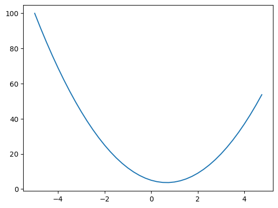
# Plot the results
plt.plot(xs, ys)

Pasted image 20231118212947

What is the derivative of the function at each x on the graph?

Of course, f'(x) = 6x - 4, but we won't do that because no one would actually write out the expression in a neural network.

This would be a huge expression, so we won't take this symbolic approach.

Definition of Derivative#

Instead, let's look at the definition of the derivative to ensure we truly understand it.

# We can basically evaluate the derivative here numerically by taking a very small h
h = 0.00000001
x = 3.0
(f(x + h) - f(x)) / h # the function responds positively

14.00000009255109

This is the function's response in the positive direction.

After normalization by the run, we have the rise over run to get the numerical approximation of the slope.

If at some position, if we push in the positive direction and the function does not respond, remaining almost unchanged, that is why slope=0.

What Derivatives Can Tell Us#

Let's look at a more complex example:

a = 2.0
b = -3.0
c = 10
d = a * b + c
print(d)

The output variable d of this function is a function of three scalar inputs, and we need to re-examine the derivatives of d with respect to a, b, and c.

h = 0.0001

# inputs
a = 2.0
b = -3.0
c = 10
d1 = a * b + c
a += h
d2 = a * b + c

print('da',d1)
print('d2',d2)
print('slope', (d2 - d1) / h)

Here, we need to feel how d2 changes after pushing a

We find that a is positive, b is negative, and as a increases, it will reduce the contribution to d, so we can expect the function value d2 to decrease.

da 4.0
d2 3.999699999999999
slope -3.000000000010772

Mathematically, it can also be proven that d(ab+c)da=b=3\frac{d(a*b+c)}{da}=b=-3

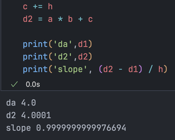
b += h

da 4.0
d2 4.0002
slope 2.0000000000042206
Screenshot 2023-11-18 at 22.00.39

The amount of increase in the function is the same as the amount we added to c, so the slope is 1.

Now that we have some intuitive understanding of how derivatives tell you about this function, we can turn to neural networks.

Framework Implementation#

Data Structure of Custom Classes#

As mentioned earlier, neural networks are very large mathematical expressions, so we need some data structures to maintain these expressions.

class Value:
    def __init__(self, data):
        self.data = data

    def __repr__(self):
        return f"Value({self.data})"

    def __add__(self, other):
        out = Value(self.data + other.data)
        return out
    
    def __mul__(self, other):
        out = Value(self.data * other.data)
        return out

a = Value(2.0)
b = Value(-3.0)
c = Value(10.0)
d = a * b + c # (a.__mul__(b)).__add__(c)

The role of repr is to provide us with a way to print output.

Now we are missing the organization of the relationships of this expression; we need to know and retain pointers about which values produced which other values.

def __init__(self, data, _children=(), _op=''):
        self.data = data
        self._prev = set(_children)
        self._op = _op

    def __repr__(self):
        return f"Value({self.data})"

    def __add__(self, other):
        out = Value(self.data + other.data, (self, other), '+')
        return out
    
    def __mul__(self, other):
        out = Value(self.data * other.data, (self, other), '*')
        return out

This way we can know the children of each value and trace back to which operation generated this value.

Now we have the complete mathematical expression and need to find a better visualization method to represent expressions that can become very large (not the focus, can be skipped).

from graphviz import Digraph

def trace(root):
    # builds a set of all nodes and edges in the graph
    nodes, edges = set(), set()
    def build(v):
        if v not in nodes:
            nodes.add(v)
            for child in v._prev:
                edges.add((child, v))
                build(child)    
    build(root)
    return nodes, edges

def draw_dot(root):
    dot = Digraph(format='svg', graph_attr={'rankdir': 'LR'}) # LR = left to right

    nodes, edges = trace(root)
    for n in nodes:
        uid = str(id(n))
        # for many values in the graph, create a rectangular ('record') node for it 
        dot.node(name = uid, label = "{ %s | data %.4f}" % (n.label, n.data), shape = 'record')
        if n._op:
            # if this value is a result of some operation, create an op node for it 
            dot.node(name = uid + n._op, label = n._op)
            # and connect this node for it 
            dot.edge(uid + n._op, uid)

    for n1, n2 in edges:
        # connect n1 to the op node of n2 
        dot.edge(str(id(n1)), str(id(n2)) + n2._op)   

    return dot

draw_dot(d)

Need to add a label member to the Value class and modify the definition as follows:

a = Value(2.0, label='a')
b = Value(-3.0, label='b')
c = Value(10.0, label='c')
e = a * b; e.label = 'e'
d = e + c; d.label = 'd'
d

Screenshot 2023-11-19 at 02.06.25

Now let's make the expression deeper:

f = Value(-2.0, label='f')
L = d * f; L.label = 'L'
L

draw_dot(L)

output 1

Visualizing forward propagation.

Running Backpropagation#

We will start from L and backtrack to compute the gradients along all intermediate values. In a neural network context, you would be very interested in the derivative of the weights of the neural network with respect to the loss function L.

In the Value class, we create a variable to maintain the derivative of L regarding that value:

self.grad = 0

At initialization, we assume that each value does not affect the output. Because a derivative of 0 means that this variable does not change the loss function.

Now we fill in the gradient starting from L; what is the derivative of L with respect to L? In other words, if I change L by a small amount h, how much will L change?

It is not hard to imagine that L will change proportionally with h, so the derivative is 1:

def lol():

    h = 0.0001
    a = Value(2.0, label='a')
    b = Value(-3.0, label='b')
    c = Value(10.0, label='c')
    e = a * b; e.label = 'e'
    d = e + c; d.label = 'd'
    f = Value(-2.0, label='f')
    L = d * f; L.label = 'L'
    L1 = L.data

    a = Value(2.0, label='a')
    b = Value(-3.0, label='b')
    c = Value(10.0, label='c')
    e = a * b; e.label = 'e'
    d = e + c; d.label = 'd'
    f = Value(-2.0, label='f')
    L = d * f; L.label = 'L'
    L2 = L.data + h

    print((L2 - L1) / h)

lol() # 0.9999999999976694
L.grad = 1.0
# L = d * f
# dL/dd = ? -> f
f.grad = 4.0 # d.data
d.grad = -2.0 # f.data

What we did with the lol() function is somewhat like an inline gradient check, which is what we do when we perform backpropagation and obtain the derivatives with respect to all intermediate results. The numerical gradient is simply an estimate using a small step size.

Now we begin to get to the essence of backpropagation; we know that L is sensitive to D, but how is L affected by C?

'''
dd / dc = ? -> 1.0 to get the local derivative
dd / de = ? -> 1.0
d = c + e

(f(x+h)) - f(x) / h 
((c + h + e) - (c + e)) / h
h / h = 1.0
'''

Calculating local derivative

The + node between c, e, and d is completely unaware of the rest of the graph; it only knows that it performed an add operation and created d, and the local influence of c and e on d. However, what we actually want is dL/dc.

How do we integrate this information to get dL/dc? The answer is the Chain Rule 链式法则

If variable z depends on variable y, and variable y depends on variable x (i.e., y and z are dependent variables), then z also depends on x through the intermediate variable y. In this case, the chain rule can be expressed as:
dzdx=dzdydydx{\displaystyle {\frac {dz}{dx}}={\frac {dz}{dy}}\cdot {\frac {dy}{dx}}}

The chain rule essentially tells you how to properly link these derivatives together.

As George F. Simmons said: “If a car is going twice as fast as a bicycle, and the bicycle is going four times as fast as a walker, then the car is going eight times faster than the person.”

This example clearly explains the core of this rule, which is Multiply.

Addition Node#

distributor of gradient

In a neural network, the operation of each node affects how gradients propagate. For an addition node, suppose there are two inputs aa and bb, which add to get c=a+bc = a + b. During backpropagation, the gradients of cc with respect to aa and bb are both 1.

Specifically:

  • If cc's gradient is Lc\frac{\partial L}{\partial c}, where LL is the loss function, then according to the chain rule, we can obtain the gradients of aa and bb:
    La=Lc×ca\frac{\partial L}{\partial a} = \frac{\partial L}{\partial c} \times \frac{\partial c}{\partial a}
    Lb=Lc×cb\frac{\partial L}{\partial b} = \frac{\partial L}{\partial c} \times \frac{\partial c}{\partial b}
  • Since c=a+bc = a + b, we have ca=1\frac{\partial c}{\partial a} = 1 and cb=1\frac{\partial c}{\partial b} = 1.
  • Therefore, both La\frac{\partial L}{\partial a} and Lb\frac{\partial L}{\partial b} equal Lc\frac{\partial L}{\partial c}.

Thus, at the addition node, the gradient is passed "as is" to all input nodes. This means that the addition node does not change the size of the gradient but distributes it evenly to all inputs. This is because the addition operation is linear for each input, and each input's contribution to the output is independent.

Multiplication Node#

To find a.grad, we can use: dL/da=(dL/de)×(de/da)=2.0×b.data=6.0dL/da=(dL/de)\times(de/da)=-2.0\times b.data=6.0

So the core idea of backpropagation can be summarized as: recursively multiply on the local derivatives.

Fine-tuning Inputs#

Fine-tuning inputs means trying to increase the value of L.

When operating on point a, it means we only need to move in the direction of the gradient.
We need to adjust the leaf nodes because, in general, we have control over them.
We expect L to increase:

a.data += 0.01 * a.grad
b.data += 0.01 * b.grad
c.data += 0.01 * c.grad
f.data += 0.01 * f.grad

e = a * b
d = e + c
L = d * f

print(L.data)

-7.286496

Using a practical example:

# inputs x1,x2
x1 = Value(2.0, label='x1')
x2 = Value(0.0, label='x2')

# weights w1,w2, the synaptic strength of each input
w1 = Value(-3.0, label='w1')
w2 = Value(1.0, label='w2')

# bias b
b = Value(6.8813735870195432, label='b')

# x1*w1 + x2*w2 + b
x1w1 = x1 * w1; x1w1.label = 'x1w1'
x2w2 = x2 * w2; x2w2.label = 'x2w2'
x1w1x2w2 = x1w1 + x2w2; x1w1x2w2.label = 'x1w1x2w2' 
n = x1w1x2w2 + b; n.label = 'n' # The original activation value of the cell body
# Now apply an activation function, here using tanh, implemented in the previous class.
def tanh(self):
        n = self.data
        t = (math.exp(2*n) - 1)/(math.exp(2*n) + 1)
        out = Value(t, (self,), 'tanh')
        return out

o = n.tanh(); o.label = 'o'
draw_dot(o)

neural

  • o.grad=1.0
  • Calculate n.grad
    o=tanh(n),do/dn=1tanh(n)2=1o2=0.5o=tanh(n),do/dn=1-tanh(n)^2=1-o^2=0.5
o.grad = 1.0
n.grad = 0.5
x1w1x2w2.grad = 0.5
b.grad = 0.5
x1w1.grad = 0.5
x2w2.grad = 0.5
x1.grad = x1w1.grad * w1.data
w1.grad = x1w1.grad * x1.data
x2.grad = x2w2.grad * w2.data 
w2.grad = x2w2.grad * x2.data

Screenshot 2023-11-22 at 15.23.20

The derivative always tells us its effect on the final output, so if I change w2, the output does not change because x2 is 0. If we want to increase the output of this neuron, w2 is not important for this neuron, but the weight of x1 should increase.

Automation#

Manually performing backpropagation is absurd; now let's see how to implement backpropagation more automatically.

We will do this by storing a special self._backward, which is a function that executes the small chain rule mentioned above, on each small node that receives input and produces output. We will store "how to link the output gradient to the input gradients."

Call the ._backward method on all nodes in topological order:

o.grad = 1.0

topo = []
visited = set()
def build_topo(v):
    if v not in visited:
        visited.add(v)
        for child in v._prev:
            build_topo(child)
        topo.append(v)
build_topo(o)

for node in reversed(topo):
    node._backward()
topo:
[Value(6.881373587019543), Value(0.0), Value(1.0), Value(0.0), Value(-3.0), Value(2.0), Value(-6.0), Value(-6.0), Value(0.8813735870195432), Value(0.7071067811865476)]

After placing this in the Value class, you only need to call o.backward() to complete the BP of a neuron.

At this point, the constructor of the Value class is as follows:

 class Value:
 '''
 data is the actual value;
 _children tuple is used to maintain child nodes for tracing;
 _op specifies the operation type
 label is used for visualization labels
 '''
    def __init__(self, data, _children=(), _op='', label=''):
        self.data = data
        self.grad = 0.0
        self._backward = lambda: None
        self._prev = set(_children)
        self._op = _op
        self.label = label

The Problem#

The current algorithm has a serious problem, but it is not apparent in the current example because each node in the example is used exactly once. If called multiple times, the currently stored gradients will be overwritten.

Screenshot 2023-11-27 at 23.17.29

The derivative is clearly 2 instead of 1.

The solution lies in the multivariate case of the chain rule and its generalization, the basic idea is to "accumulate these gradients":

self.grad += 1.0 * out.grad
other.grad += 1.0 * out.grad

Screenshot 2023-11-27 at 23.21.58

The problem is fixed.

Operation Level#

The execution operation level of the entire framework is entirely up to you:

As long as you can implement the forward and backward passes of each operation, it does not matter how complex that operation is. In other words, if you can implement local gradients, then the design of these functions is entirely up to you:

def tanh(self):
        n = self.data
        t = (math.exp(2*n) - 1)/(math.exp(2*n) + 1)
        out = Value(t, (self,), 'tanh')

        def _backward():
            self.grad += (1 - t**2) * out.grad
        out._backward = _backward

        return out

Screenshot 2024-01-16 at 22.28.40

Using tanh.

# Need to implement BP for all atomic operations.
def __repr__(self):
        return f"Value({self.data})"

    def __add__(self, other):
        other = other if isinstance(other, Value) else Value(other)
        out = Value(self.data + other.data, (self, other), '+')

        def _backward():
            self.grad += 1.0 * out.grad
            other.grad += 1.0 * out.grad
        out._backward = _backward

        return out

    def __sub__(self, other):
        return self + (-other)

    def __radd__(self, other): # r means reverse, used to implement reverse operations for defined operations, allowing custom class objects to better interact with Python's operators and built-in types.
        return self.__add__(other)
    
    def __mul__(self, other):
        other = other if isinstance(other, Value) else Value(other)
        out = Value(self.data * other.data, (self, other), '*')

        def _backward():
            self.grad += other.data * out.grad
            other.grad += self.data * out.grad
        out._backward = _backward

        return out
    
    def __pow__(self, other):
        assert isinstance(other, (int, float)), "only supporting int/float powers for now"
        out = Value(self.data**other, (self,), f'**{other}')

        def _backward():
            self.grad += other * self.data ** (other - 1) * out.grad
        out._backward = _backward

        return out

    def __rmul__(self, other):
        return self.__mul__(other)
    
    def __truediv__(self, other):
        return self * other**-1

Screenshot 2024-01-16 at 22.30.21

Using e2x1/e2x+1e^{2x}-1/{e^{2x}+1}

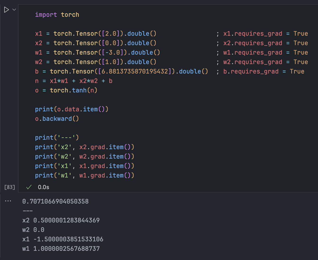
Corresponding Implementation in Torch#

Screenshot 2024-01-17 at 14.49.08

Implementation of Neuron Class#

^c9c15a

import random

class Neuron:
    def __init__(self, nin):
        self.w = [Value(random.uniform(-1,1)) for _ in range(nin)]
        self.b = Value(random.uniform(-1,1))

    def __call__(self, x):
        # w * x + b
        act = sum((wi * xi for wi, xi in zip(self.w,x)), self.b)
        out = act.tanh()
        return out
    
x = [2.0, 3.0]
n = Neuron(2)
n(x)

Implementing MLP#

^da5567

Pasted image 20240117145319

You can see that each layer has multiple neurons that are not interconnected but are all connected to the input.
So a Layer is a group of independently evaluated neurons.

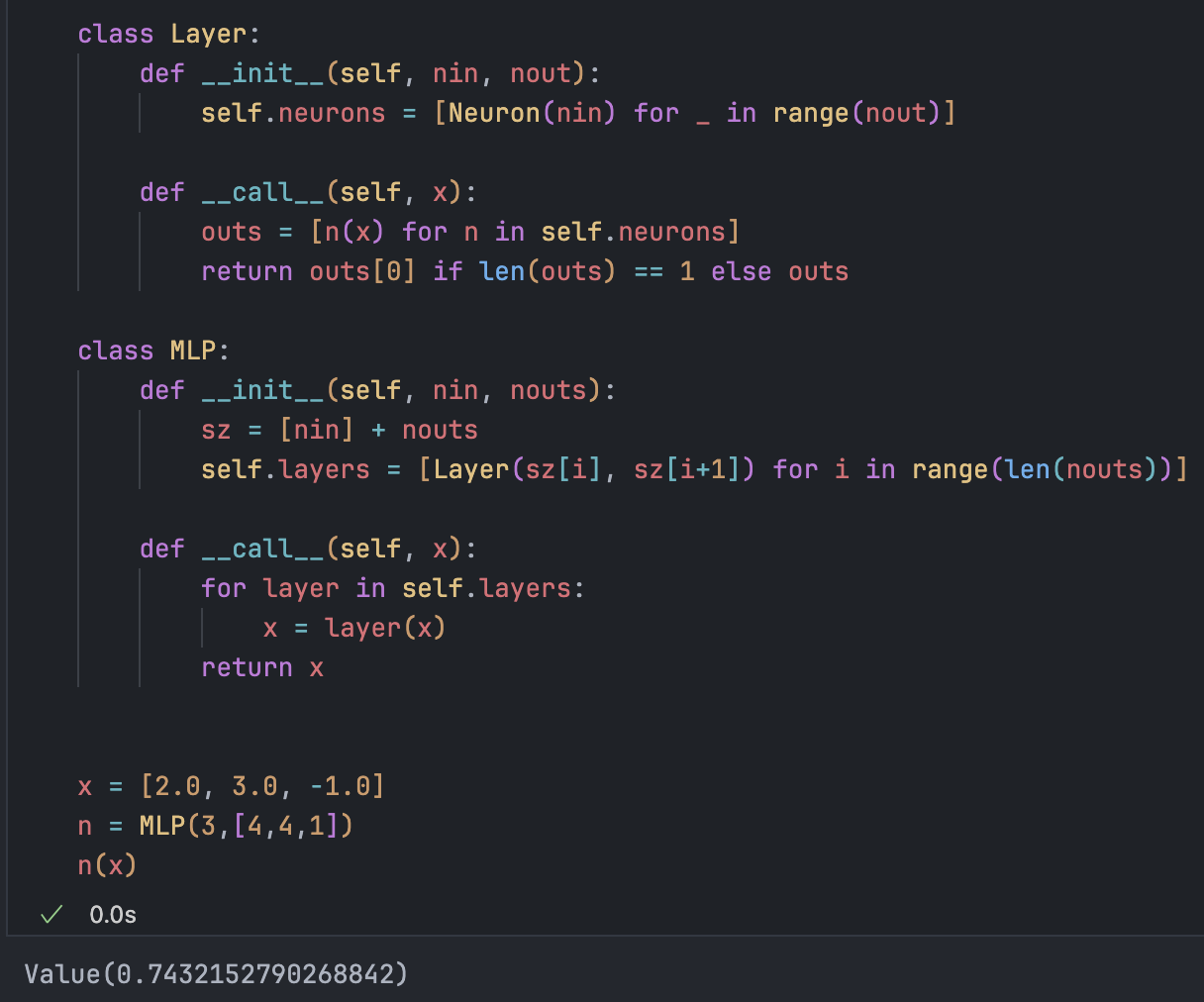
First, implement a single Layer:

Screenshot 2024-01-17 at 15.04.56

Implement MLP according to the diagram:

Screenshot 2024-01-17 at 15.21.39

3 inputs, two layers of 4 neurons, 1 output.

Define a simple dataset where we want the neural network to perform binary classification on the four samples in xs, obtaining the results in ys:

Screenshot 2024-01-17 at 15.24.27

Clearly, the results cannot reach the target.

So how can we build a neural network that can adjust weights to better predict the desired targets?
The trick to achieving this in deep learning is to compute a single number that somehow measures the overall performance of the neural network, which is the loss (the loss).

In classic machine learning algorithms, this number corresponds to the mean squared error (MSE) used in generalized linear models, which serves to measure the performance of the model.

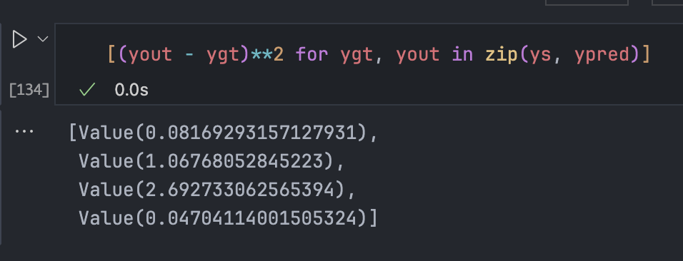
Screenshot 2024-01-17 at 15.34.28

First, observe the loss for each group; it can be seen that as a loss, MSE only equals 0 when y output = y true value. The further the prediction deviates, the larger the loss becomes.

Thus, we arrive at the final loss: which is the sum of all losses:

Screenshot 2024-01-17 at 15.37.07

Store weights and biases:

Screenshot 2024-01-17 at 15.48.37

Both writing styles have the same effect.

Similarly, implement for the MLP class:

def parameters(self):
        return [p for layer in self.layers for p in layer.parameters()]

Screenshot 2024-01-17 at 15.52.07

Here we can change the weights based on the gradient information. But here we can see that if we increase w[0].data, because its gradient is negative at this time, it will actually decrease it, and the loss will rise.

Screenshot 2024-01-17 at 15.55.46

So the current gradient descent lacks a -, which means "moving in the negative direction of the gradient" to minimize the loss.

for p in n.parameters():
	p.data += - 0.01 * p.grad*

It can be seen that the loss indeed decreased, and our prediction effect improved somewhat:

Screenshot 2024-01-17 at 16.02.59

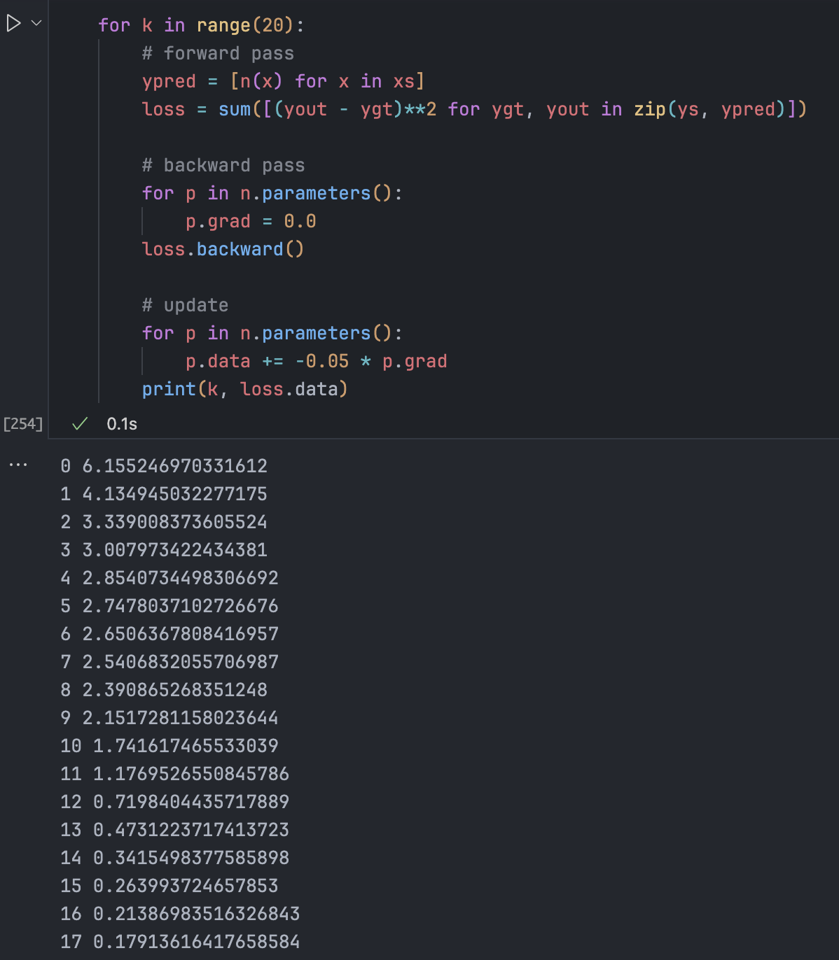
Now what is needed is to iterate this process; the calculation of the loss function is called the "Forward Pass," then backpropagate again, update the data, and this will yield a lower loss.

The above is the "gradient descent" process in neural networks: forward propagation, backpropagation, and updating data, during which the neural network gradually improves its prediction performance.

If you try to change the step size, you may exceed the appropriate bounds. Because we basically do not understand the current loss function, our only knowledge is the local dependency between these parameters and the loss function. If the step is too large, it may enter a completely different part of the loss function, leading to gradient explosion and other issues.

In the current case, after several iterations, the loss has approached 0, and it can be seen that the results in ypred are already quite good (the learning rate or step size is set to 0.1).

Screenshot 2024-01-17 at 16.13.30

Upon executing again, gradient explosion occurs (loss rises above 5), and the prediction effect is extremely poor:

Screenshot 2024-01-17 at 16.15.43
But in the next iteration, the effect is exceptionally good:

Screenshot 2024-01-17 at 16.17.17

It can be seen that the setting and adjustment of the learning rate is a subtle art. Too low requires a long time to converge, while too high can lead to instability. Therefore, in ordinary gradient descent, the setting of the step size is indeed a science.

Common Problems in Neural Networks#

In the previous process, there was actually a huge problem; it was only because the problem we analyzed was too simple that we did not discover where the loophole was.

Because the gradients defined earlier are cumulative, we need to perform a zero grad operation before each backpropagation; otherwise, it is equivalent to increasingly large steps, making it difficult to achieve the desired result.

Adding gradient clearing during the iteration process, it can be seen that the convergence speed is slower now and cannot reach a low loss in just a few steps, which is the normal situation:

Screenshot 2024-01-17 at 16.30.44

This bug may not affect much at times, but when facing complex problems, it can lead to poor optimization of the loss.

The common mistakes listed, the one just encountered is the 3rd:

Pasted image 20240117163412

Summary: What is a Neural Network?#

A neural network is a mathematical expression, and in the case of multiple layers, it is a relatively simple formula, taking data, the weights and parameters of the neural network as input; the forward propagation is a mathematical expression, followed by the loss function, which measures the accuracy of the prediction, and then backpropagates the loss, operating according to the gradient information to minimize the loss.

We only need a bunch of neurons to make it do anything; the neural network in the current example has only 41 parameters, but you can build more complex neural networks with billions of neurons. Take the GPT model as an example, we have a large amount of text from the internet, trying to get the neural network to predict the next word in a sequence based on some words; this is the problem it needs to learn. Such a large neural network will have many interesting properties and hundreds of billions of parameters, but it essentially operates on the same principles, except that the update method is slightly different, and the loss function uses cross-entropy loss to predict the next token.

The current micrograd library differs from the example, as the current use is ReLU as the activation function, while here tanh is used because it is smoother and a bit more complex, emphasizing local gradients and using these derivatives.

To match the nn.module class API in PyTorch, all neuron classes in the project inherit from a parent class Module, which has the effect of zeroing gradients:

class Module:
	def zero_grad(self):
		for p in self.parameters():
		p.grad = 0.0

	def parameters(self):
		return [] 

	class Neuron(Module):
		...

Learning the implementation of micrograd helps to understand the basic design philosophy of PyTorch, making it easy to understand how to register a function type into PyTorch for automated gradient computation. The official documentation can be found here.

Loading...
Ownership of this post data is guaranteed by blockchain and smart contracts to the creator alone.