
Building the Transformer architecture from scratch, deeply understanding core components like self-attention, multi-head attention, residual connections, and layer normalization.
History of LLM Evolution (5): Building the Path of Self-Attention — The Future of Language Models from Transformer to GPT
Prerequisites: Previous micrograd and makemore series (optional), familiarity with Python, basic concepts of calculus and statistics.
Goal: Understand and appreciate how GPT works.
Resources you might need: Colab Notebook Link Detailed notes found on Twitter
ChatGPT
From the debut of ChatGPT in late 2022 to today’s GPT-4 and Claude 3, Large Language Models (LLMs) have integrated into the daily lives of many. They are probabilistic systems; for the same prompt, their answers vary. Compared to the language models we built previously, GPT can model sequences of words, characters, or more general symbols, knowing how words in English tend to follow each other. From these models’ perspective, our prompt is the beginning of a sequence, and the model’s job is to complete it.
So, what is the neural network that models these word sequences?
Transformer
In 2017, the milestone paper 《Attention is All You Need》 proposed the Transformer architecture. GPT, which we know well, stands for Generative Pre-trained Transformer. Although the original paper targeted machine translation, its profound impact has reached the entire AI field. Minor modifications to this architecture allow it to be applied to a vast array of AI applications, and it is the core of ChatGPT.
Of course, our goal isn’t to train a ChatGPT—that’s a massive industrial project involving enormous data training, pre-training, and fine-tuning. We aim to train a Transformer-based language model, which, like our previous ones, will be character-level.
Building the Model
Dataset
We’ll use the toy-scale “Tiny Shakespeare” dataset, a favorite of Andrej Karpathy. It’s a collection of Shakespeare’s works, roughly 1MB in size. Note that while ChatGPT outputs tokens (chunks of words), we’ll start with characters.
# Always start with a dataset. Download Tiny Shakespeare.
!wget https://raw.githubusercontent.com/karpathy/char-rnn/master/data/tinyshakespeare/input.txt
# Read to check
with open('input.txt', 'r', encoding='utf-8') as f:
text = f.read()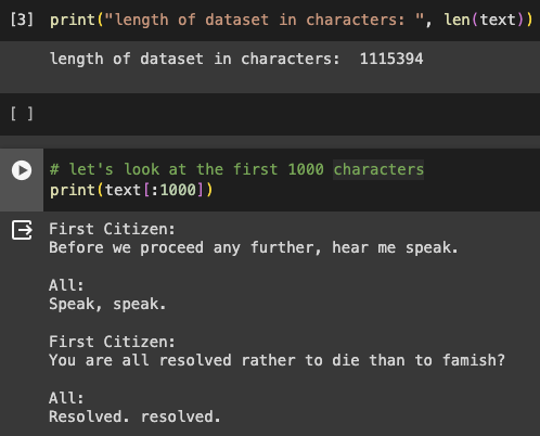
Tokenize
chars = sorted(list(set(text))) # Get unique characters and sort them
vocab_size = len(chars)
print(''.join(chars)) # Merge into one string
print(vocab_size)
# Output (Sorted by ASCII):
# !$&',-.3:;?ABCDEFGHIJKLMNOPQRSTUVWXYZabcdefghijklmnopqrstuvwxyz
# 65This character table logic is identical to our previous sections. We then need a way to tokenize the input—converting the raw text string into a sequence of integers. For our character-level model, this just means mapping each character to a number.
If you’ve followed the previous sections, this code should feel familiar, much like the lookup table in Bigram.
# Map characters to integers
stoi = { ch:i for i,ch in enumerate(chars) }
itos = { i:ch for i,ch in enumerate(chars) }
encode = lambda s: [stoi[c] for c in s] # encoder: string to list of integers
decode = lambda l: ''.join([itos[i] for i in l]) # decoder: list of integers to string
print(encode("hii there"))
print(decode(encode("hii there")))We’ve built an encoder and decoder to translate between strings and integers at the character level. This is a very simple tokenization algorithm. Many methods exist, like Google’s SentencePiece, which splits text into subwords (commonly used in practice), and OpenAI’s TikToken, which uses byte pairs.
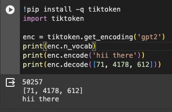
Using tiktoken: GPT-2’s vocabulary has 50,257 tokens. For the same string, it uses only 3 integers compared to our simple algorithm.
# Encode the entire dataset into a torch.tensor
import torch
data = torch.tensor(encode(text), dtype=torch.long)
print(data.shape, data.dtype)
print(data[:1000]) In GPT, the first 1000 characters look like this:


As seen, 0 is space and 1 is a newline.
Currently, the entire dataset is represented as a massive sequence of integers.
Train/Val Split
# Split data into training and validation sets to check for overfitting
n = int(0.9*len(data)) # First 90% for training, rest for validation
train_data = data[:n]
val_data = data[n:]We don’t want the model to perfectly memorize Shakespeare; we want it to learn his style.
Chunks & Batches
We won’t feed the entire text into the Transformer at once. Instead, we’ll use random chunks (samples) from the training set.
Chunking
Block Size specifies the fixed length of each input data chunk.
block_size = 8
train_data[:block_size+1]
x = train_data[:block_size]
y = train_data[1:block_size+1]
for t in range(block_size):
context = x[:t+1]
target = y[t]
print(f"when input is {context} the target: {target}")
This strategy gradually reveals context to the model.
This forces the model to learn to predict the next character based on preceding ones, improving reasoning ability.
Batching
To utilize GPU parallelism, we pile multiple text chunks into a single tensor, processing independent data blocks simultaneously.
The batch size determines how many independent sequences the Transformer processes in one forward/backward pass.
torch.manual_seed(1337) # For reproducibility
batch_size = 4 # Number of independent sequences to process in parallel
block_size = 8 # Max context length for prediction
# Similar to torch DataLoader
def get_batch(split):
# Generate a small batch of inputs x and targets y
data = train_data if split == 'train' else val_data
ix = torch.randint(len(data) - block_size, (batch_size,))
x = torch.stack([data[i:i+block_size] for i in ix])
y = torch.stack([data[i+1:i+block_size+1] for i in ix])
return x, y
xb, yb = get_batch('train')
torch.stackconcatenates tensors along a new dimension.
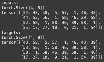
xb shape is 4x8, with each row being a chunk from the training set. yb targets are used to calculate the loss function.
for b in range(batch_size): # Batch dimension
for t in range(block_size): # Time dimension
context = xb[b, :t+1]
target = yb[b,t]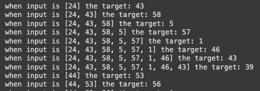
This clarifies the relationship between inputs and outputs.
Bigram
We previously implemented a Bigram language model in Makemore; now we’ll reimplement it quickly using torch.nn.Module.
Model Construction
import torch
import torch.nn as nn
from torch.nn import functional as F
torch.manual_seed(1337)
class BigramLanguageModel(nn.Module):
super().__init__()
# Each token reads logits for the next token directly from a lookup table
self.token_embedding_table = nn.Embedding(vocab_size, vocab_size)The embedding layer is familiar: if the input is 24, it retrieves the 24th row of the table.
def forward(self, idx, targets=None):
# idx and targets are (B, T) tensors of integers
logits = self.token_embedding_table(idx) # (Batch=4, Time=8, Channel=65)
if targets is None:
loss = None
else:
B, T, C = logits.shape
logits = logits.view(B*T, C)
targets = targets.view(B*T)
loss = F.cross_entropy(logits, targets)
return logits, lossWe know negative log-likelihood is a good loss measure, implemented as “cross-entropy” in PyTorch. Intuitively, the model should assign a high probability to the correct label and very low probabilities elsewhere. The expected loss is roughly -log(1/65) ≈ 4.17, though actual results are slightly higher due to entropy.
# Generation from the model
def generate(self, idx, max_new_tokens):
# idx is (B, T) array of indices in current context
for _ in range(max_new_tokens):
# Get predictions
logits, loss = self(idx)
# Focus only on the last time step
logits = logits[:, -1, :] # Becomes (B, C)
# Apply softmax for probabilities
probs = F.softmax(logits, dim=-1) # (B, C)
# Sample from distribution
idx_next = torch.multinomial(probs, num_samples=1) # (B, 1)
# Append sampled index to sequence
idx = torch.cat((idx, idx_next), dim=1) # (B, T+1)
return idx
print(loss)
print(decode(m.generate(idx = torch.zeros((1, 1), dtype=torch.long), max_new_tokens=100)[0].tolist())) # Start with newline (0)generate expands the context idx from BxT to across all batches in the time dimension.

Random output from an untrained model.
Model Training
We’ll use the popular AdamW optimizer instead of Makemore’s SGD.
# Create PyTorch optimizer
optimizer = torch.optim.AdamW(m.parameters(), lr=1e-3)The optimizer computes gradients and updates parameters.
batch_size = 32 # Larger batch size
for steps in range(100): # Increase steps for better results
# Sample a batch
xb, yb = get_batch('train')
# Evaluate loss
logits, loss = m(xb, yb)
optimizer.zero_grad(set_to_none=True) # Clear previous gradients
loss.backward() # Backpropagation
optimizer.step() # Update parameters
print(loss.item())
Optimization is working; loss is decreasing.
With more training, loss reached ~2.48. Sampling again yields better results.
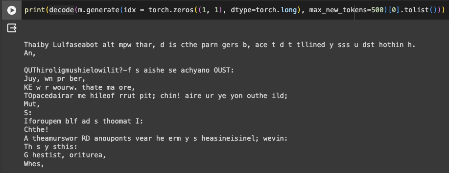
Better, but still not quite right.
Bigram models are limited because they only predict based on the single previous token. There’s no connection between tokens further back, hence the need for Transformers.
Transformer
If you have an NVIDIA GPU, you can accelerate training:
device = 'cuda' if torch.cuda.is_available() else 'cpu'Setting this requires adjusting code to ensure data loading, computation, and sampling happen on the GPU. See Andrej’s lecture repository for the starting bigram.py.
We’ve split the model into training and evaluation phases. Currently, only nn.Embedding exists, so both phases behave identically. Adding dropout or batch norm layers later makes this split crucial—a best practice in model training.
Self-Attention
Before the full Transformer, we’ll learn a mathematical trick for implementing self-attention.
torch.manual_seed(1337)
B,T,C = 4,8,2 # batch, time, channels
x = torch.randn(B,T,C)
# x.shape = torch.Size([4, 8, 2])We want tokens to interact specifically: e.g., the 5th token shouldn’t “see” tokens 6, 7, or 8 because they are in the future. It only communicates with tokens 1-4. Information flows from previous context to the current step to predict the future.
The simplest way for tokens to communicate? Averaging preceding tokens to form a historical feature vector. However, this loses spatial arrangement information.
v1. For Loop
# Target: x[b,t] = mean_{i<=t} x[b,i]
xbow = torch.zeros((B,T,C))
for b in range(B):
for t in range(T):
xprev = x[b,:t+1] # (t,c)
xbow[b,t] = torch.mean(xprev, 0)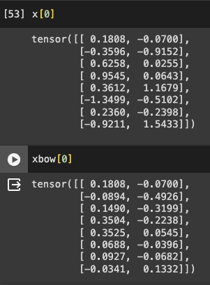
The code calculates cumulative averages.
This is inefficient. Matrix multiplication can do this better.
v2. Matrix Multiplication
# Simplified example: weighted aggregation using matrix multiplication.
torch.manual_seed(42)
a = torch.ones(3, 3)
b = torch.randint(0,10,(3,2)).float()
c = a @ bStandard matrix multiplication: each element in c is the dot product of a row from a and a column from b.
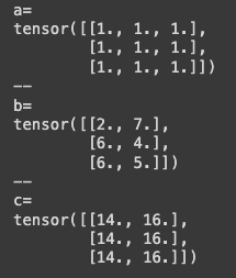
To achieve our goal, use a lower triangular matrix:
This sums the first rows, implemented via torch.tril.
a = torch.tril(torch.ones(3, 3))Normalize each row so they sum to 1 for weighted aggregation:
a = torch.tril(torch.ones(3, 3))
a = a / torch.sum(a, 1, keepdim=True) # keepdim for broadcasting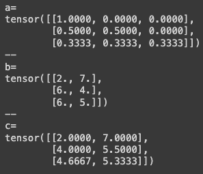
Each row sums to 1;
cis now the mean of preceding rows inb.
Applying this:
# v2: Weighted aggregation via matrix multiplication
wei = torch.tril(torch.ones(T, T))
wei = wei / wei.sum(1, keepdim=True) 
The weight matrix corresponds to matrix
aabove.
# torch adds a batch dimension to wei
xbow2 = wei @ x # (T, T) @ (B, T, C) ----> (B, T, C)
torch.allclose(xbow, xbow2) # True: same effectSummary: Batch matrix multiplication with a lower triangular weight matrix performs weighted aggregation, where token only sees tokens t$.
v3. Softmax
We can also use Softmax for a third version.
torch.masked_fill() fills a tensor based on a mask:
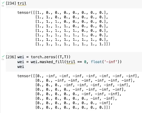
Applying Softmax to each row performs the same weighted aggregation:
# v3: Using Softmax
tril = torch.tril(torch.ones(T, T))
wei = torch.zeros((T,T))
wei = wei.masked_fill(tril == 0, float('-inf'))
wei = F.softmax(wei, dim=-1)
xbow3 = wei @ xBeyond encoding identity, we encode position:
class BigramLanguageModel(nn.Module):
super().__init__()
# Tokens read logits from a lookup table
self.token_embedding_table = nn.Embedding(vocab_size, n_embd) # token encoding
self.position_embedding_table = nn.Embedding(block_size, n_embd) # position encoding
def forward(self, idx, targets=None):
B, T = idx.shape
# idx and targets are (B,T) integer tensors
tok_emb = self.token_embedding_table(idx) # (B,T,C)
pos_emb = self.position_embedding_table(torch.arange(T, device=device)) # (T,C)
x = tok_emb + pos_emb # (B,T,C)
x = self.blocks(x) # (B,T,C)
x = self.ln_f(x) # (B,T,C)
logits = self.lm_head(x) # (B,T,vocab_size)x stores the sum of token and position embeddings. In Bigram, positions are translationally invariant, but that changes with attention.
v4. Self-Attention
Simple averaging treats all tokens equally. In reality, tokens have different meanings—they are data-dependent. For example, a vowel might want to “know” which consonants precede it. Self-attention solves this.
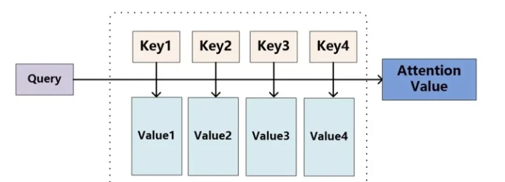
Each token emits two vectors: a query (what am I looking for?) and a key (what do I contain?).
Affinity (weights) between tokens is the dot product of keys and queries. High alignment results in a high weight, focusing the model’s attention on that specific token’s information.
Attention computes matches between queries and keys to assign weights, allowing the model to focus on the most relevant information.
We also need a Value (what information do I contribute if you’re interested in me?). We aggregate these values (passed through a linear layer) instead of raw x.
Implementing single-head self-attention:
# v4: self-attention!
torch.manual_seed(1337)
B,T,C = 4,8,32 # batch, time, channels
x = torch.randn(B,T,C)
# Single-head self-attention
head_size = 16
key = nn.Linear(C, head_size, bias=False)
query = nn.Linear(C, head_size, bias=False)
value = nn.Linear(C, head_size, bias=False)
k = key(x) # (B, T, 16)
q = query(x) # (B, T, 16)
# Dot product for affinities
wei = q @ k.transpose(-2, -1) # (B, T, 16) @ (B, 16, T) ---> (B, T, T)
tril = torch.tril(torch.ones(T, T))
wei = wei.masked_fill(tril == 0, float('-inf'))
wei = F.softmax(wei, dim=-1)
v = value(x)
out = wei @ v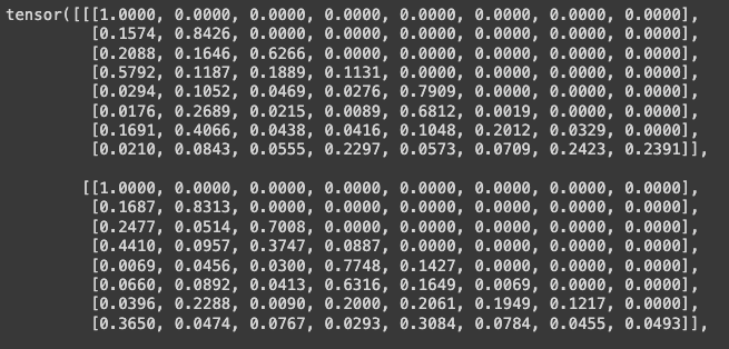
weiweights are now data-dependent: tokens with high affinity contribute more information.
Attention Summary
Attention is a communication mechanism. Nodes in a directed graph aggregate information from connected nodes via weighted sums, where weights are data-dependent.
It lacks spatial concepts. Attention acts on a set of vectors, which is why position encoding is necessary.
Batch examples are handled independently.
Attention doesn’t strictly care about the past. Our implementation masks future information using
masked_fill, but removing it allows all-to-all communication (Encoder style). Ours is a “Decoder” module due to the triangular mask.“Self-attention” means keys and values come from the same source as the query (
x). “Cross-attention” uses queries fromxbut keys/values from an external source (e.g., an encoder).“Scaled” Attention: Divide
weiby .

With unit Gaussian inputs, raw weighted sum wei has variance proportional to the head size.
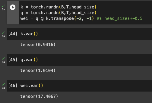
Normalization brings variance back to 1:
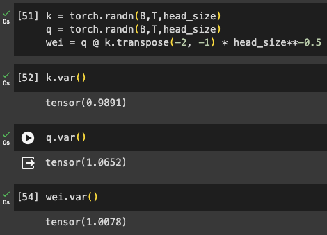
Why does this matter? Softmax makes distributions with large absolute values more “peaky” (approaching one-hot).

Scaling controls initialization variance, keeping Softmax diffuse and preventing gradient issues.
Code Implementation
class Head(nn.Module):
""" one head of self-attention """
def __init__(self, head_size):
super().__init__()
self.key = nn.Linear(n_embd, head_size, bias=False)
self.query = nn.Linear(n_embd, head_size, bias=False)
self.value = nn.Linear(n_embd, head_size, bias=False)
self.register_buffer('tril', torch.tril(torch.ones(block_size, block_size)))
def forward(self, x):
B,T,C = x.shape
k = self.key(x) # (B,T,C)
q = self.query(x) # (B,T,C)
# Compute affinities, apply scaling
wei = q @ k.transpose(-2,-1) * C**-0.5 # (B, T, C) @ (B, C, T) -> (B, T, T)
wei = wei.masked_fill(self.tril[:T, :T] == 0, float('-inf')) # (B, T, T)
wei = F.softmax(wei, dim=-1) # (B, T, T)
# Weighted aggregation
v = self.value(x) # (B,T,C)
out = wei @ v # (B, T, T) @ (B, T, C) -> (B, T, C)
return outtril is a buffer, not a parameter, so we use register_buffer.
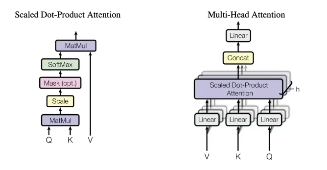
Multi-Head Attention
Multi-head attention applies multiple heads in parallel and concatenates results:
Code Implementation
In PyTorch, just create a list of heads.
class MultiHeadAttention(nn.Module):
""" Multiple heads of self-attention in parallel. """
def __init__(self, num_heads, head_size):
super().__init__()
self.heads = nn.ModuleList([Head(head_size) for _ in range(num_heads)])
def forward(self, x):
return torch.cat([h(x) for h in self.heads], dim=-1) # Concatenate on channel dimWe now have multiple communication channels. It’s similar to group convolution.
class BigramLanguageModel(nn.Module):
def __init__(self):
super().__init__()
self.token_embedding_table = nn.Embedding(vocab_size, n_embd)
self.position_embedding_table = nn.Embedding(block_size, n_embd)
self.sa_heads = MultiHeadAttention(4, n_embd//4)
self.lm_head = nn.Linear(n_embd, vocab_size)Blocks
The Transformer architecture repeats blocks containing multi-head attention and a feed-forward part.
Feed-Forward Network
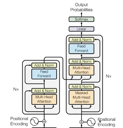
The feed-forward part is a simple MLP:
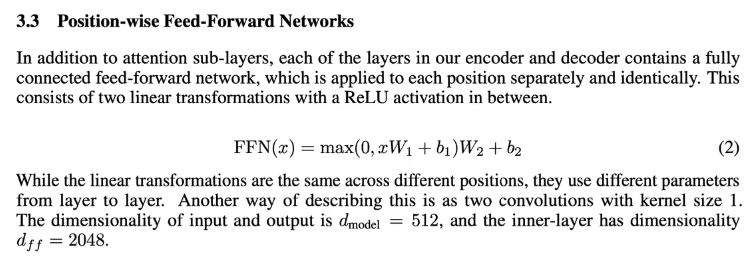
The paper uses 512 for IO and 2048 for the inner layer, so we multiply inner channel size by 4.
class FeedForward(nn.Module):
""" Simple linear layer followed by non-linearity """
def __init__(self, n_embd):
super().__init__()
self.net = nn.Sequential(
nn.Linear(n_embd, 4 * n_embd),
nn.ReLU(),
)
def forward(self, x):
return self.net(x)
class Block(nn.Module):
""" Transformer block: decouples communication and computation """
def __init__(self, n_embd, n_head):
super().__init__()
head_size = n_embd // n_head
self.sa = MultiHeadAttention(n_head, head_size) # Communication
self.ffwd = FeedForward(n_embd) # Computation
def forward(self, x):
x = self.sa(x)
x = self.ffwd(x)
return x
class BigramLanguageModel(nn.Module):
def __init__(self):
super().__init__()
self.token_embedding_table = nn.Embedding(vocab_size, n_embd)
self.position_embedding_table = nn.Embedding(block_size, n_embd)
self.blocks = nn.Sequential(
Block(n_embd, n_head=4),
Block(n_embd, n_head=4),
Block(n_embd, n_head=4),
)
self.lm_head = nn.Linear(n_embd, vocab_size)Adding blocks doesn’t immediately improve decoding much. We’ve created a deep network that suffers from optimization issues. We need solutions from the paper.
Residual Connections
Residual connections (Skip connections) were proposed in Deep Residual Learning for Image Recognition.
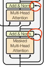
Andrej: “You transform data, then have a skip connection and add it from the previous features.”

- Transform data: Data undergoes weights and non-linearities to learn abstract representations.
- Skip connection: Break sequential patterns by connecting inputs directly to later layers.
- Addition: Element-wise addition ensures original features propagate without being “diluted.”
Residual connections facilitate learning identity mappings, crucial for deep networks. They allow gradients to flow directly, mitigating vanishing/exploding gradients.
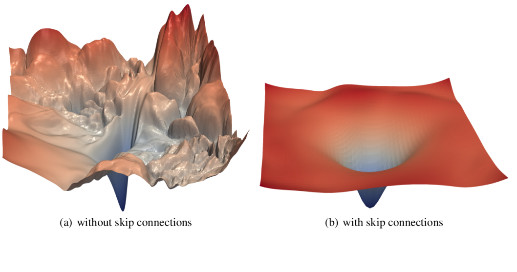
In micrograd, we saw addition nodes distribute gradients equally to all inputs. Everything is connected.
class MultiHeadAttention(nn.Module):
def __init__(self, num_heads, head_size):
super().__init__()
self.heads = nn.ModuleList([Head(head_size) for _ in range(num_heads)])
self.proj = nn.Linear(n_embd, n_embd) # Projection
def forward(self, x):
out = torch.cat([h(x) for h in self.heads], dim=-1)
out = self.proj(out) # Linear transformation for residual path
return out
class FeedForward(nn.Module):
def __init__(self, n_embd):
super().__init__()
self.net = nn.Sequential(
nn.Linear(n_embd, 4 * n_embd),
nn.ReLU(),
nn.Linear(4 * n_embd, n_embd), # Project back to residual path
)
def forward(self, x):
return self.net(x)
class Block(nn.Module):
def __init__(self, n_embd, n_head):
super().__init__()
head_size = n_embd // n_head
self.sa = MultiHeadAttention(n_head, head_size)
self.ffwd = FeedForward(n_embd)
def forward(self, x):
x = x + self.sa(x) # Residual addition
x = x + self.ffwd(x)
return xLayer Norm
The second optimization is Layer Norm:
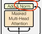
Similar to Batch Norm, but normalizes across features instead of the batch dimension. It computes mean and std for all features of each sample. While the original paper applies it after transformation, modern practice uses “Pre-norm”—applying Layer Norm before the transformation.
We now have a fairly complete Transformer (decoder-only).
class Block(nn.Module):
def __init__(self, n_embd, n_head):
super().__init__()
head_size = n_embd // n_head
self.sa = MultiHeadAttention(n_head, head_size)
self.ffwd = FeedForward(n_embd)
self.ln1 = nn.LayerNorm(n_embd)
self.ln2 = nn.LayerNorm(n_embd)
def forward(self, x):
x = x + self.sa(self.ln1(x))
x = x + self.ffwd(self.ln2(x))
return x
class BigramLanguageModel(nn.Module):
def __init__(self):
super().__init__()
self.token_embedding_table = nn.Embedding(vocab_size, n_embd)
self.position_embedding_table = nn.Embedding(block_size, n_embd)
self.blocks = nn.Sequential(*[Block(n_embd, n_head=n_head) for _ in range(n_layer)])
self.ln_f = nn.LayerNorm(n_embd) # Final Layer Norm
self.lm_head = nn.Linear(n_embd, vocab_size)Dropout
Dropout randomly shuts off neurons during forward/backward passes to prevent overfitting, as proposed in Dropout: A Simple Way to Prevent Neural Networks from Overfitting.
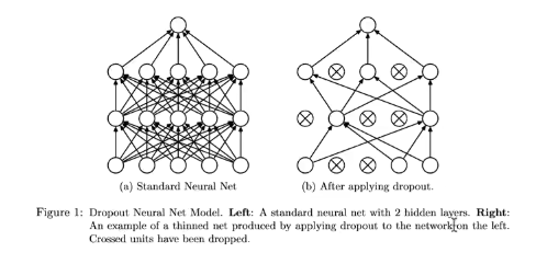
# Hyperparameters
batch_size = 64
block_size = 256 # Context length
max_iters = 5000
learning_rate = 1e-3
device = 'cuda' if torch.cuda.is_available() else 'cpu'
n_embd = 384
n_head = 6
n_layer = 4
dropout = 0.2
class Head(nn.Module):
def __init__(self, head_size):
super().__init__()
self.key = nn.Linear(n_embd, head_size, bias=False)
self.query = nn.Linear(n_embd, head_size, bias=False)
self.value = nn.Linear(n_embd, head_size, bias=False)
self.register_buffer('tril', torch.tril(torch.ones(block_size, block_size)))
self.dropout = nn.Dropout(dropout)
def forward(self, x):
# ... same as before
wei = F.softmax(wei, dim=-1)
wei = self.dropout(wei) # Dropout on attention weights
# ...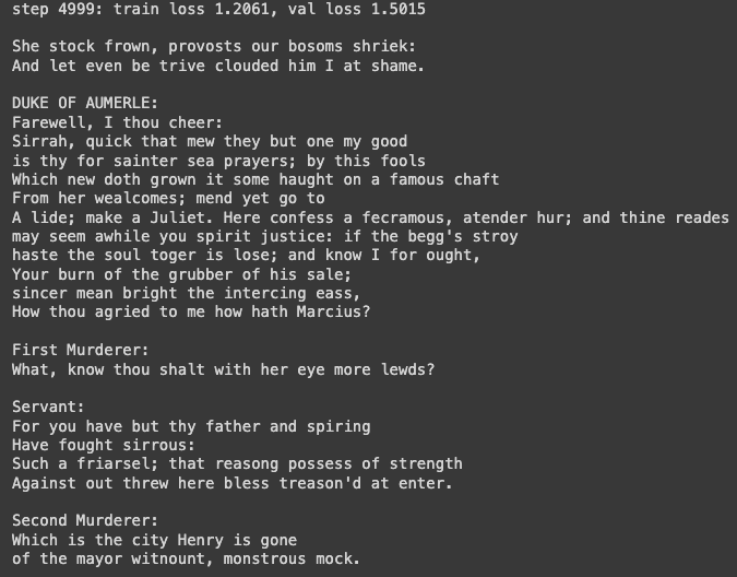
The output looks like Shakespearean gibberish, quite impressive for a small model.
We didn’t implement the encoder or cross-attention from the original paper.
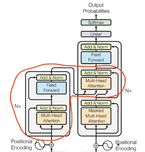
We use decoder-only because we’re generating unconditional text. The triangular mask ensures autoregressive property for language modeling.
The original paper’s encoder-decoder structure is for translation: encoding a sentence (e.g., French) and decoding it into English.

See karpathy/nanoGPT for a decoder-only pre-training implementation.
Back to ChatGPT
Training ChatGPT involves two stages: pre-training and fine-tuning.
Pre-training
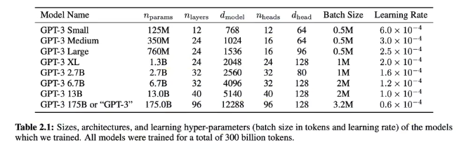
Train on a massive Internet corpus to get an encoder-only Transformer. OpenAI uses tokenizers (byte pairs). Our Shakespeare model has ~10M parameters; GPT-3 has 175B, trained on 300B tokens.
After this, the model only completes sequences; it can’t answer questions.
Fine-tuning
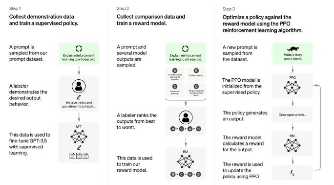
- Alignment: Fine-tune on thousands of “Question: Answer” documents.
- Reward Model: Humans rank model responses.
- PPO: Use Proximal Policy Optimization to fine-tune the sampling policy, turning the document completer into a chatbot.
Andrej’s Microsoft Build 2023 talk provides a comprehensive overview: State of GPT.