History of LLM Evolution (4): WaveNet — Convolutional Innovation in Sequence Models

The source code repository for this section.

In previous sections, we built a character-level language model using a Multi-Layer Perceptron (MLP). Now, it’s time to make its structure more complex. Our current goal is to allow more characters in the input sequence (currently 3). Furthermore, we don’t want to squeeze all of them into a single hidden layer to avoid over-compressing information. This leads us to a deeper model similar to WaveNet.

WaveNet

Published in 2016, WaveNet is essentially a language model, but it predicts audio sequences instead of character or word-level sequences. Fundamentally, the modeling setup is the same—both are Autoregressive Models trying to predict the next element in a sequence.

The paper uses a hierarchical tree structure for prediction, which we will implement in this section.

nn.Module

We’ll encapsulate the previous content into classes, mimicking the PyTorch nn.Module API. This allows us to think of modules like “Linear,” “1D Batch Norm,” and “Tanh” as Lego bricks used to build neural networks:

class Linear:
  
  def __init__(self, fan_in, fan_out, bias=True):
    self.weight = torch.randn((fan_in, fan_out), generator=g) / fan_in**0.5
    self.bias = torch.zeros(fan_out) if bias else None
  
  def __call__(self, x):
    self.out = x @ self.weight
    if self.bias is not None:
      self.out += self.bias
    return self.out
  
  def parameters(self):
    return [self.weight] + ([] if self.bias is None else [self.bias])

Linear layer module: Its role is to perform a matrix multiplication during the forward pass.

class BatchNorm1d:
  
  def __init__(self, dim, eps=1e-5, momentum=0.1):
    self.eps = eps
    self.momentum = momentum
    self.training = True
    # Parameters trained via backpropagation
    self.gamma = torch.ones(dim)
    self.beta = torch.zeros(dim)
    # Buffers trained via "momentum updates"
    self.running_mean = torch.zeros(dim)
    self.running_var = torch.ones(dim)
  
  def __call__(self, x):
    # Calculate forward pass
    if self.training:
      xmean = x.mean(0, keepdim=True) # Batch mean
      xvar = x.var(0, keepdim=True) # Batch variance
    else:
      xmean = self.running_mean
      xvar = self.running_var
    xhat = (x - xmean) / torch.sqrt(xvar + self.eps) # Normalize data to unit variance
    self.out = self.gamma * xhat + self.beta
    # Update buffers
    if self.training:
      with torch.no_grad():
        self.running_mean = (1 - self.momentum) * self.running_mean + self.momentum * xmean
        self.running_var = (1 - self.momentum) * self.running_var + self.momentum * xvar
    return self.out
  
  def parameters(self):
    return [self.gamma, self.beta]

Batch-Norm:

1. Has running_mean & running_var updated outside of backpropagation.
2. self.training = True: Since batch norm behaves differently in training vs. evaluation, we need a training flag to track its state.
3. Performs coupled calculations on elements within a batch to control activation statistics and reduce Internal Covariate Shift.

class Tanh:
  def __call__(self, x):
    self.out = torch.tanh(x)
    return self.out
  def parameters(self):
    return []

Instead of a local torch.Generator g, we’ll set a global random seed:

torch.manual_seed(42);

The following should look familiar, including the embedding table C and our layer structure:

n_embd = 10 # Dimension of character embedding vectors
n_hidden = 200 # Number of neurons in the MLP hidden layer
 
C = torch.randn((vocab_size, n_embd))
layers = [
	Linear(n_embd * block_size, n_hidden, bias=False), 
	BatchNorm1d(n_hidden), 
	Tanh(),
	Linear(n_hidden, vocab_size),
]
 
# Initialize parameters
with torch.no_grad():
	layers[-1].weight *= 0.1 # Scale down the last layer (output layer) to reduce initial confidence
 
parameters = [C] + [p for layer in layers for p in layer.parameters()]
'''
List comprehension, equivalent to:
for layer in layers:
	for p in layer.parameters():
		p...
'''
 
print(sum(p.nelement() for p in parameters)) # total number of parameters
for p in parameters:
  p.requires_grad = True

The optimization training part remains unchanged for now. We notice the loss function curve has high fluctuations because a batch size of 32 is too small—each batch can be very “lucky” or “unlucky” (high noise).

During evaluation, we must set the training flag to False for all layers (currently only affecting batch norm):

# Set layers to evaluation mode
for layer in layers:
	layer.training = False

Let’s fix the loss function visualization:

lossi is a list of all losses. We’ll average the values inside to get a more representative curve.

Reviewing torch.view():

Equivalent to view(5, -1)

This is convenient for unfolding values in a list.

torch.tensor(lossi).view(-1, 1000).mean(1)

Looks much better now. We can observe the learning rate reduction reaching local minima.

Next, we turn the previous Embedding and Flattening operations into modules:

emb = C[Xb]
x = emb.view(emb.shape[0], -1)

class Embedding:
  
  def __init__(self, num_embeddings, embedding_dim):
    self.weight = torch.randn((num_embeddings, embedding_dim))
    # C now becomes embedding weights
    
  def __call__(self, IX):
    self.out = self.weight[IX]
    return self.out
  
  def parameters(self):
    return [self.weight]
 
 
class FlattenConsecutive:
    
  def __call__(self, x):
    self.out = x.view(x.shape[0], -1)
    return self.out
  
  def parameters(self):
    return []

PyTorch has a container concept, essentially a way to organize layers as lists or dictionaries. Sequential is one such container that passes input through all layers in order:

class Sequential:
  
  def __init__(self, layers):
    self.layers = layers
  
  def __call__(self, x):
    for layer in self.layers:
      x = layer(x)
    self.out = x
    return self.out
  
  def parameters(self):
    # Get parameters from all layers and flatten into a list
    return [p for layer in self.layers for p in layer.parameters()]

Now we have a Model concept:

model = Sequential([
  Embedding(vocab_size, n_embd),
  Flatten(),
  Linear(n_embd * block_size, n_hidden, bias=False),
  BatchNorm1d(n_hidden), Tanh(),
  Linear(n_hidden, vocab_size),
])
 
parameters = model.parameters()
print(sum(p.nelement() for p in parameters)) # total parameter count
for p in parameters:
  p.requires_grad = True

This yields further simplification:

# forward pass
  logits = model(Xb)
  loss = F.cross_entropy(logits, Yb) # loss function
 
# evaluate the loss
  logits = model(x)
  loss = F.cross_entropy(logits, y)
 
# sample from the model
  # forward pass the neural net 
  logits = model(torch.tensor([context]))
  probs = F.softmax(logits, dim=1)

Implementing the Hierarchical Structure

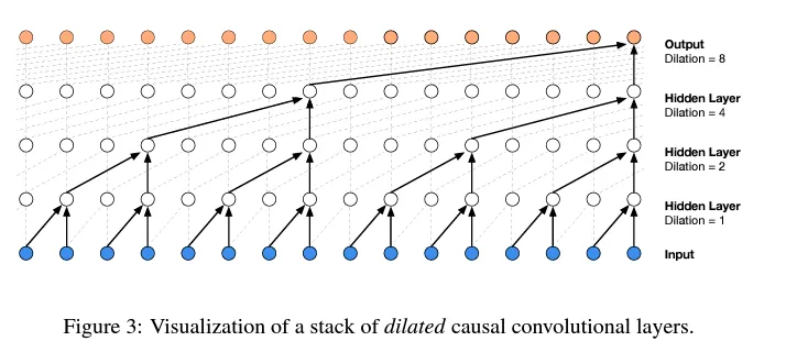
We don’t want to squeeze all information into one layer in one step like our current model. Instead, like WaveNet, we want to predict the next character by fusing two characters into a two-character representation, then into four-character blocks, and so on, progressively fusing information into the network through a hierarchical tree structure.

In WaveNet, this diagram visualizes a “Dilated causal convolution layer.” Don’t worry about the specifics; we are focusing on the core idea: Progressive fusion.

Increase context input and process these 8 characters in a tree structure:

# block_size = 3
# train 2.0677597522735596; val 2.1055991649627686
block_size = 8

Simply expanding the context length improves performance:

To understand what we’re doing, let’s observe the tensor shapes as they pass through layers:

Inputting 4 random numbers with block_size=8 gives a shape of 4x8.

1. After the first layer (embedding), we get a 4x8x10 output—meaning our embedding table has a learned 10D vector for each character.
2. After the second layer (flatten), it becomes 4x80. This layer stretches the 10D embeddings of these 8 characters into one long row, like a concatenation operation.
3. The third layer (linear) uses matrix multiplication to turn these 80 numbers into 200 channels.

To recap what the Embedding layer does:

This answer explains it perfectly:

1. Turns a sparse matrix into a dense matrix through linear transformation (table lookup).
2. This dense matrix uses N features to represent all words. Coefficients represent relationships between words and features, encapsulating deep relationships between words.
3. The weights are encoding parameters learned by the embedding layer, which are continuously optimized during backpropagation.

A linear layer takes input X, multiplies it by weights, and optionally adds a bias:

def __init__(self, fan_in, fan_out, bias=True):
    self.weight = torch.randn((fan_in, fan_out)) / fan_in**0.5 # note: kaiming init
    self.bias = torch.zeros(fan_out) if bias else None

Weights are 2D, bias is 1D.

Based on input/output shapes, the linear layer looks like this internally:

(torch.randn(4, 80) @ torch.randn(80, 200) + torch.randn(200)).shape

Output is 4x200. Bias addition follows broadcasting semantics.

Note that PyTorch matrix multiplication supports high-dimensional tensors, operating only on the last dimension while treating others as batch dimensions.

This is very useful for our next goal: parallel batch dimensions. Instead of inputting 80 numbers at once, we want two characters fused together in the first layer—inputting 20 numbers, like so:

# (1 2) (3 4) (5 6) (7 8)
 
(torch.randn(4, 4, 20) @ torch.randn(20, 200) + torch.randn(200)).shape

This becomes four sets of bigrams, each a 10D vector.

To implement this, Python provides a convenient way to slice even and odd parts of a list:

e = torch.randn(4, 8, 10)
torch.cat([e[:, ::2, :], e[:, 1::2, :]], dim=2)
# torch.Size([4, 4, 20])

This explicitly extracts even and odd parts and concatenates the two 4x4x10 parts together.

The powerful view() can do equivalent work.

Now, let’s refine our Flatten layer. Create a constructor that takes the number of consecutive elements we want to concatenate in the last dimension.

class FlattenConsecutive:
  
  def __init__(self, n):
    self.n = n
    
  def __call__(self, x):
    B, T, C = x.shape
    x = x.view(B, T//self.n, C*self.n)
    if x.shape[1] == 1:
      x = x.squeeze(1)
    self.out = x
    return self.out
  
  def parameters(self):
    return []

• B: Batch size, number of samples.
• T: Time steps, length of the sequence.
• C: Channels or Features per time step.

1. Input Tensor: Input x is a 3D tensor of shape (B, T, C).

2. Flattening Operation: By calling x.view(B, T//self.n, C*self.n), the class merges consecutive time steps. self.n is the number of steps to merge. This results in each new time step being a wider feature vector containing information from n original steps. Time dimension T is reduced by n, while feature dimension C is increased by n.

3. Removing Unit Dimension: If the resulting time dimension is 1 (x.shape[1] == 1), x.squeeze(1) removes it, bringing us back to the 2D case we saw before.

Check the shapes of intermediate layers after the change:

In batch norm, we want to maintain mean and variance for only 68 channels, not 32x4 dimensions. So we update the BatchNorm1d implementation:

class BatchNorm1d:
  
  def __call__(self, x):
    # calculate the forward pass
    if self.training:
      if x.ndim == 2:
        dim = 0
      elif x.ndim == 3:
        dim = (0,1) # torch.mean() can take a tuple of dimensions
        
      xmean = x.mean(dim, keepdim=True) # batch mean
      xvar = x.var(dim, keepdim=True) # batch variance

Now running_mean.shape is [1, 1, 68].

Scaling Up the Network

With the improvements complete, we now further increase performance by increasing network size.

n_embd = 24    # Embedding dimension
n_hidden = 128 # Number of neurons in MLP hidden layer

Parameter count reaches 76,579, and performance breaks the 2.0 barrier:

By now, training time has significantly increased. Despite performance gains, setting hyperparameters like learning rate still feels like blind debugging, constantly monitoring training loss.

Convolution

In this section, we implemented the main architecture of WaveNet but didn’t implement the specific forward pass involving more complex gated linear layers, Residual connections, and Skip connections.

Let’s briefly understand how our tree structure relates to the Convolutional Neural Networks used in the WaveNet paper.

Essentially, we use Convolution for efficiency. It allows us to slide the model over the input sequence, performing the loops (sliding the kernel and calculating) within CUDA kernels.

We implemented a single black structure from the diagram to get one output, but convolution lets you apply this black structure across the input sequence, calculating all orange outputs simultaneously like a linear filter.

Efficiency gains:

1. Loops are done in CUDA cores.
2. Variable reuse: For example, a white dot in the second layer is both the left child of one third-layer dot and the right child of another. The node value is used twice.

Summary

After this section, the torch.nn module is unlocked, and we will transition to using it for future model implementations.

Reflecting on this section, a lot of time was spent getting layer shapes right. Andrej always debugs shapes in a Jupyter Notebook before copying the satisfied code into VS Code.