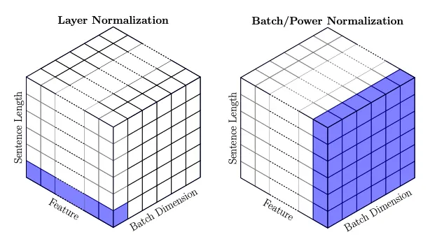
Deeply understand the activation and gradient issues in neural network training, and learn how batch normalization solves the training challenges of deep networks.
History of LLM Evolution (3): Batch Normalization — Statistical Harmony of Activations and Gradients
The focus of this section is to gain a deep impression and understanding of neural network activations, especially the downward-flowing gradients during training. Understanding the historical development of these structures is crucial because RNNs (Recurrent Neural Networks), as universal approximators, can theoretically implement any algorithm but are difficult to optimize using gradient-based techniques. The reason for this difficulty is a key point of understanding, which can be concluded by observing the behavior of activations and gradients during training. We will also see many variants that attempt to improve this situation.
Starting Point: MLP
Let’s revisit the MLP model from the previous chapter, which is our current starting point. We’ll modify the code from the last chapter to avoid hard-coding, making it easier to adjust later.
# MLP revisited
n_embd = 10 # Dimension of character embedding vectors
n_hidden = 200 # Number of hidden units in the hidden layer
# vocab_size = 27, block_size = 3
g = torch.Generator().manual_seed(2147483647) # for reproducibility
C = torch.randn((vocab_size,n_embd), generator=g)
W1 = torch.randn((n_embd * block_size, n_hidden), generator=g)
b1 = torch.randn(n_hidden, generator=g)
W2 = torch.randn((n_hidden, vocab_size), generator=g)
b2 = torch.randn(vocab_size, generator=g)
parameters = [C, W1, b1, W2, b2]
print(sum(p.nelement() for p in parameters)) # Total parameters
for p in parameters:
p.requires_grad_()The total parameter count is 11,897, same as the last chapter.
The training part of the neural network is also modified without changing functionality:
# Same mini-batch optimization as the last chapter
max_steps = 200000
batch_size = 32
lossi = []
for i in range(max_steps):
# mini-batch
ix = torch.randint(0,Xtr.shape[0],(batch_size,), generator=g)
Xb, Yb = Xtr[ix], Ytr[ix] # batch X, Y
# forward pass
emb = C[Xb] # embedding
embcat = emb.view(emb.shape[0], -1) # Concatenate all embedding vectors
hpreact = embcat @ W1 + b1 # Hidden layer pre-activation
h = torch.tanh(hpreact) # Hidden layer
logits = h @ W2 + b2 # Output layer
loss = F.cross_entropy(logits, Yb) # Loss function
# backward pass
for p in parameters:
p.grad = None
loss.backward()
# update
lr = 0.1 if i < 100000 else 0.01
for p in parameters:
p.data += -lr * p.grad
# tracks stats
if i % 10000 == 0:
print(f'{i:7d}/{max_steps:7d}: {loss.item():.4f}')
lossi.append(loss.log10().item())
plt.plot(lossi)
Note that the initial loss is as high as 27, then drops very quickly. Can you guess why?
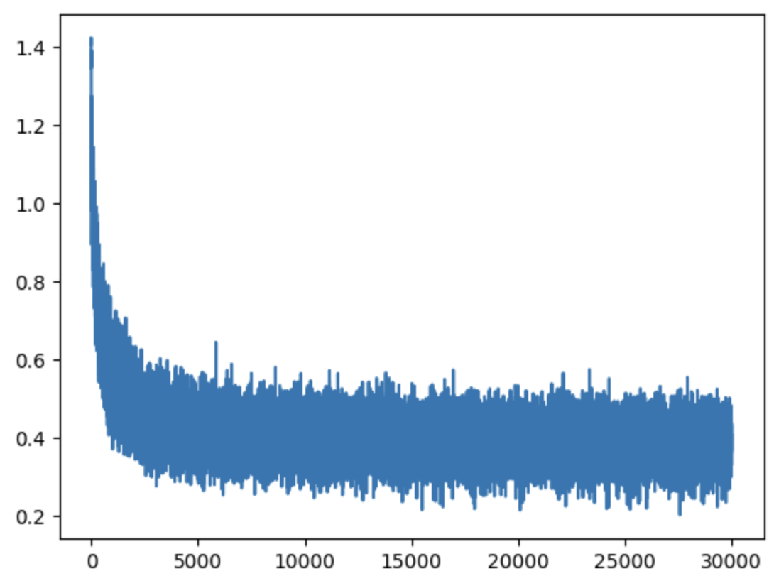
Looks like a hockey stick.
Loss visualization also includes a feature to split loss by index for different parts:
@torch.no_grad() # This decorator cancels gradient tracking inside this function
def split_loss(split):
x,y = {
'train': (Xtr, Ytr),
'val': (Xdev, Ydev),
'test': (Xte, Yte),
}[split]
# forward pass
emb = C[x] # (N, block_size, n_embd)
embcat = emb.view(emb.shape[0], -1) # Concatenate to (N, block_size * n_embd)
h = torch.tanh(embcat @ W1 + b1) # (N, n_hidden)
logits = h @ W2 + b2 # (N, vocab_size)
loss = F.cross_entropy(logits, y)
print(split, loss.item())
split_loss('train')
split_loss('val')This decorator acts like setting
requires_grad = Falsefor every tensor and preventsbackward()calls, avoiding the overhead of maintaining the computational graph.
The losses here are: train 2.2318217754364014 val 2.251192569732666
# sample from the model
g = torch.Generator().manual_seed(2147483647 + 10)
for _ in range(20):
out = []
context = [0] * block_size # initialize with all ...
while True:
# Forward pass
emb = C[torch.tensor([context])] # (1, block_size, n_embd)
h = torch.tanh(emb.view(1, -1) @ W1 + b1)
logits = h @ W2 + b2
probs = F.softmax(logits, dim=1)
# Sample from distribution
ix = torch.multinomial(probs, num_samples=1, generator=g).item()
# Slide context window and track sample
context = context[1:] + [ix]
out.append(ix)
# Break if special '.' terminator is sampled
if ix == 0:
break
print(''.join(itos[i] for i in out))Sampling results:
carlah. amorilli. kemri. rehty. sacessaeja. huteferniya. jareei. nellara. chaiir. kaleig. dham. jore. quint. sroel. alian. quinaelon. jarynix. kaeliigsat. edde. oia.The performance isn’t great yet, but it’s better than the Bigram model.
Initialization Fixes
First, as mentioned, the initial loss was way too high, indicating a problem with the neural network’s initialization step.
What do we want at initialization?
There are 27 possible next characters, and we have no reason to assume any character is more likely than others. So we expect an initial uniform distribution (1/27). Let’s manually calculate the correct initial loss:
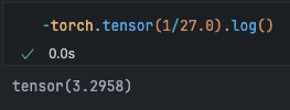
Much smaller than 27.
The high initial loss is caused by the large gaps in probability distributions between characters due to random network assignment. We can check this with breakpoints:
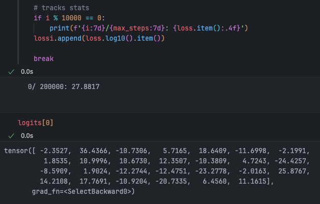
Logits should all be roughly 0. Such extreme distributions cause false confidence, leading to large losses.
Since logits are defined as h @ W2 + b2, we can make these parameters smaller:
W2 = torch.randn((n_hidden, vocab_size), generator=g) * 0.01
b2 = torch.randn(vocab_size, generator=g) * 0
Logits are now close to 0.
Very close to the desired loss (3.2985 mentioned above).
Could we set W2 to exactly 0 to get the minimum loss?
You don’t want to set neural network weights to exactly 0, as this leads to symmetry breaking problems, hindering the network from learning useful features. So we just set it to a very small number.
The current loss still has some entropy, called symmetry breaking.

Let’s see how
devv.aiexplains this term. By the way, this site is great.
Removing the break and verifying our optimization yielded the expected results:
0/ 200000: 3.3221
10000/ 200000: 2.1900
...
190000/ 200000: 1.9368
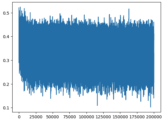
train 2.123051404953003 val 2.163424015045166
The initial loss is now normal, the graph is no longer a hockey stick, and final performance is better. The improvement is because we spent more cycles optimizing the network instead of the first few thousand iterations compressing excessively high initial weights.
Gradient Vanishing
Visualizing h and hpreact:

We see many hidden layer activations distributed at ±1, caused by pre-activations being spread over too large a range (tanh output saturates at ±1 for large absolute inputs).
This is actually bad. Recall the tanh implementation and its backpropagation in micrograd: tanh only reduces gradients by a certain proportion. At tanh units where , our gradient vanishes. This is because tanh is in the flat tail when output is near ±1, having little impact on loss, so the gradient is 0. If is 0, the neuron is active (gradient is passed through unchanged).
def tanh(self):
# ... forward pass code
def _backward():
self.grad += (1 - t**2) * out.grad
out._backward = _backward
return outIf all examples in a neuron are ±1, that neuron isn’t learning at all; it’s a “dead neuron.”
Observing that no neuron is completely white (abs value > 0.99 = True), neurons will still learn, but we certainly want fewer pre-activations at ±1 during initialization.
This also applies to other nonlinear activation functions like Sigmoid, which also acts as a squashing function. For ReLU, gradient vanishing occurs when pre-activation is negative, setting the gradient to zero during backpropagation. Besides occurring at initialization, if the learning rate is too high, neurons might receive very large gradient updates, pushing weights to extreme values where they no longer activate for any input (output always 0). This is called being “knocked out,” becoming a dead neuron—like permanent brain damage. The commonly used ELU also has this problem.
Leaky ReLU doesn’t have this issue because it lacks a flat tail, always providing a gradient.
Weight Initialization
The source of the problem, hpreact, is embedding multiplied by , which is too far from 0. What we want is very similar to our expectations for logits:
W1 = torch.randn((n_embd * block_size, n_hidden), generator=g) * 0.1
b1 = torch.randn(n_hidden, generator=g) * 0.01
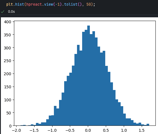
The histogram is much better now because the pre-activation range was reduced to (-2, 1.5).

Now there are no neurons above 0.99.
Increasing the W1 coefficient to 0.2 gave satisfactory results:

Original: train 2.2318217754364014 val 2.251192569732666
Fixed overconfident softmax: train 2.123051404953003 val 2.163424015045166
Fixed saturated tanh at initialization: train 2.035430431365967 val 2.1064531803131104
Despite poor initialization, the network learned some features. This is only because this single-layer MLP is shallow and the optimization problem is simple and forgiving. In deeper networks, these issues would be severe.
How do we set these scaling factors for large, deep networks?
Initialization Strategy
Let’s observe what happens to the mean and standard deviation when multiplying two Gaussian distributions during pre-activation.
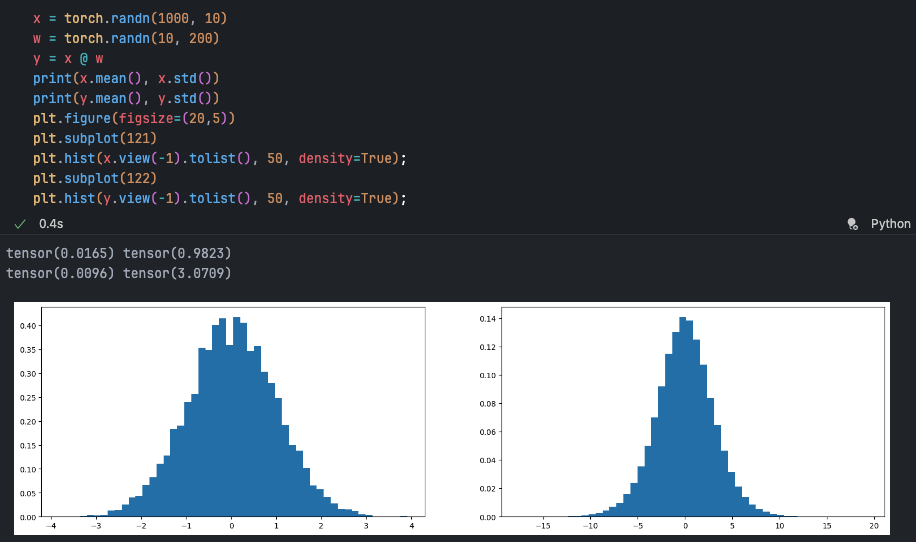
The mean is still near 0 due to symmetry, but the standard deviation tripled, so the Gaussian distribution is expanding.
In neural networks, we want activation distributions at each layer to not differ too much at initialization to avoid vanishing or exploding gradients. Wide or narrow distributions lead to instability. Ideally, the network should have a good initial activation distribution to ensure information and gradients propagate effectively.
This corresponds to the concept of Internal Covariate Shift.
What’s the right scaling factor?
w = torch.randn(10, 200) * 0.3
'''
tensor(-0.0237) tensor(1.0103)
tensor(-0.0005) tensor(0.9183)
Already close. How to get exactly a standard normal distribution?
'''Weight initialization usually normalizes initial values such that weights are divided by the square root of their input connection count (fan-in).
x = torch.randn(1000, 10)
w = torch.randn(10, 200) / 10**0.5 # input element count is 10
A widely cited paper on this is Delving Deep into Rectifiers: Surpassing Human-Level Performance on Image Net Classification. It specifically studied ReLU and P-ReLU nonlinearities in CNNs. Since ReLU zeroes out negative activations, essentially discarding half the distribution, you need to compensate during the forward pass. Research found that weights must be initialized with a zero-mean Gaussian with standard deviation , whereas we used , precisely because ReLU discards half the distribution.
This is built into PyTorch, see torch.nn.init:
torch.nn.init.kaiming_normal_(tensor, a=0, mode='fan_in', nonlinearity='leaky_relu', generator=None)Parameters for this function:
tensor: Tensor to be initialized.a: Mean of the normal distribution, default 0.mode: Mode for calculating std, ‘fan_in’ or ‘fan_out’, default ‘fan_in’. ‘fan_in’ for inputs, ‘fan_out’ for outputs.nonlinearity: Type of nonlinear activation function, defaulttorch.nn.functional.relu.

According to the paper, different nonlinearities have different corresponding gains:
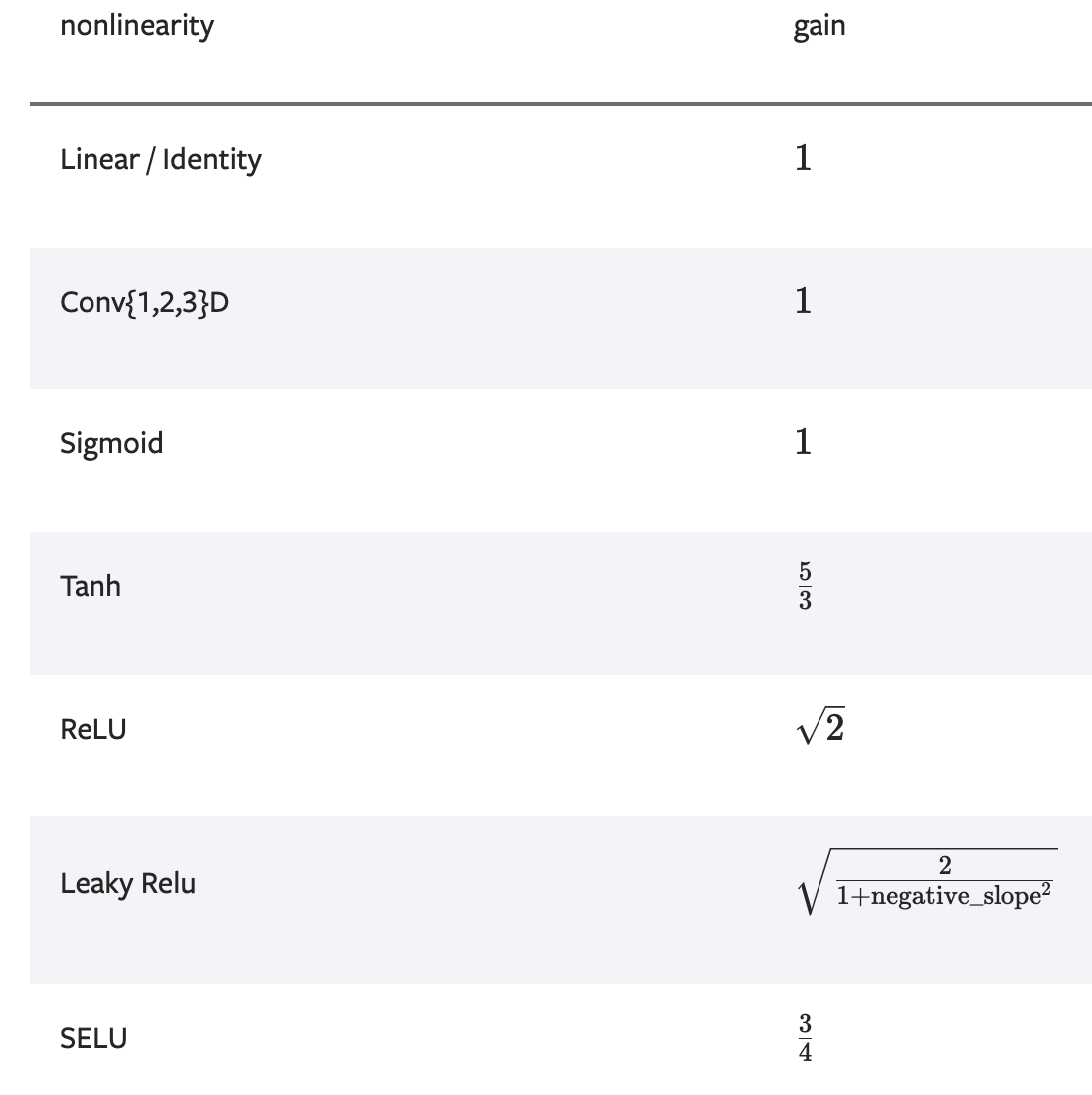
The ReLU gain here corresponds to the mentioned above.
The tanh we use also needs such a gain because, just as ReLU squashes negatives to 0, tanh squashes tails. We need to prevent the gain from this squashing operation to return the distribution to standard normal.
Years ago, neural networks were very fragile regarding initialization. However, modern innovations like Residual Networks, various normalization layers, and better optimizers (Adam, etc.) have made “guaranteeing perfect initialization” relatively less important.
In practice, we modify the previous gain according to the formula :
W1 = torch.randn((n_embd * block_size, n_hidden), generator=g) * (5/3)/((n_embd * block_size)**0.5) # 0.2Re-training yielded similar results.
Batch Norm
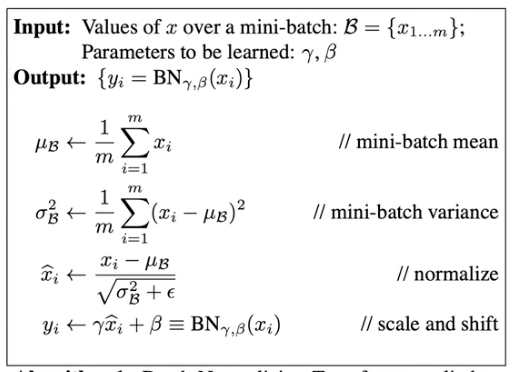
The influential Batch Normalization was proposed by a Google team in 2015, making it possible to train deep networks. The core idea is that you can directly correct hidden states (corresponding to our hpreact) to a standard normal distribution.
hpreact = embcat @ W1 + b1 # Hidden layer pre-activation
hpreact = (hpreact - hpreact.mean(0, keepdim=True)) / hpreact.std(0, keepdim=True) # batch normalizationThis ensures that even in deep networks, the firing rate (activation value) of each neuron remains in an approximate Gaussian distribution favorable for gradient descent optimization during initialization. Later, backpropagation needs to tell us how this distribution should transform—becoming sharper or more dispersed—making some neurons more “trigger-happy” (active) or harder to activate.
Thus, we also have a scale and shift step, adding gain and bias to the normalized distribution to get the layer output.
# Adding parameters
bngain = torch.ones((1, n_hidden))
bnbias = torch.zeros((1, n_hidden))
parameters = [C, W1, b1, W2, b2, bngain, bnbias]
# scale and shift
hpreact = bngain * (hpreact - hpreact.mean(0, keepdim=True)) / hpreact.std(0, keepdim=True) + bnbias # batch normalizationAt initialization, gain and bias are 1 and 0, giving the standard normal distribution we want. Since they are differentiable, they can be backpropagated during optimization.
Performance after adding batch norm layer: train 2.0668270587921143 val 2.104844808578491
Not much change, as this is a simple example with one hidden layer. We could directly calculate the weight matrix () scale to make hpreact roughly Gaussian; batch norm doesn’t do much here. But in deeper systems with many operations, adjusting weight scales would be very difficult. Uniformly adding batch norm layers across different levels makes it much easier. It’s common practice to append a batch norm layer after linear or convolution layers to control activation scales at every point.
Batch Normalization works well in practice and has some Regularization side effects, effectively controlling activations and distributions. Since batch selection is random, it introduces extra “entropy,” reducing the risk of overfitting.
Andrej Karpathy mentions that batch normalization is mathematically “coupled,” meaning it makes statistical distributions across layers interdependent. We split into multiple batches for efficiency, but normalization for each point in a batch depends on the batch mean and variance, leading to several issues:
Batch Dependency: Batch norm depends on small batch statistics, meaning performance can be affected by batch size. Mean and variance estimates for small batches can have high variance, leading to unstable training.
Domain Shift: Data distributions can differ significantly across domains (e.g., train vs. inference). Batch norm needs consistent behavior across domains. This is usually solved by using a moving average of the full training set’s mean and variance for inference.
Coupled Gradients: Calculating gradients for a batch norm layer requires considering the whole batch, meaning gradients for individual points are no longer independent. This coupling might limit gradient direction and magnitude during optimization.
For these reasons, researchers look for alternatives like Linear Normalization, Layer Normalization, Group Normalization, and Instance Normalization.
Inference Issues with Batch Norm
During training, mean and std for each batch are calculated in real-time to normalize the current batch. However, during inference, we typically process one sample at a time or use a different batch size. We cannot use single-sample statistics for batch norm as it leads to high variance and unstable predictions.
To solve this, the paper proposed having batch-norm calculate a moving average of the whole dataset’s mean and variance during training. These are then used during inference to replace batch statistics. This ensures the model uses stable statistics calculated on training data regardless of inference batch size.
# Calibrating batch norm after training
with torch.no_grad():
# Pass training set through
emb = C[Xtr]
embcat = emb.view(emb.shape[0], -1)
hpreact = embcat @ W1 + b1
# Calculate mean and std
bnmean = hpreact.mean(0, keepdim=True)
bnstd = hpreact.std(0, keepdim=True)When evaluating on training and validation sets, replace dynamic std and mean with our calculated overall averages:
# hpreact = bngain * (hpreact - hpreact.mean(0, keepdim=True)) / hpreact.std(0, keepdim=True) + bnbias
hpreact = bngain * (hpreact - bnmean) / bnstd + bnbiasNow we can also perform inference on single examples.
In reality, nobody wants a separate second stage for mean/std estimation. The paper suggests an alternative: estimating these values using a running average during training.
First, define and initialize the running versions:
# BatchNorm parameters
bngain = torch.ones((1, n_hidden))
bnbias = torch.zeros((1, n_hidden))
bnmean_running = torch.zeros((1, n_hidden))
bnstd_running = torch.ones((1, n_hidden))As mentioned, we initialized W1 and b1 to ensure pre-activations are roughly standard Gaussian, so mean is ~0 and std is ~1.
# BatchNorm layer
# -------------------------------------------------------------
bnmeani = hpreact.mean(0, keepdim=True)
bnstdi = hpreact.std(0, keepdim=True)
hpreact = bngain * (hpreact - bnmeani) / bnstdi + bnbiasWe update them during training. In PyTorch, these means and stds are not optimized via gradient descent; we never derive gradients for them.
with torch.no_grad():
bnmean_running = 0.999 * bnmean_running + 0.001 * bnmeani
bnstd_running = 0.999 * bnstd_running + 0.001 * bnstdi
# -------------------------------------------------------------0.999 and 0.001 are examples of decay factors in a moving average. They define the relative importance of past vs. new values:
- 0.999 (
momentum) is the decay factor, deciding how much of the previously accumulated running mean/variance to keep. - 0.001 (1 - momentum) is the weight for the new batch mean/variance.
The paper also includes this step:

For example, $$ defaults to , basically to prevent division by 0, corresponding to the eps parameter in BATCHNORM1D.
One more thing is unnecessary:
# Linear layer
hpreact = embcat @ W1 # + b1 removed bias here # pre-activation
# BatchNorm layer
bnmeani = hpreact.mean(0, keepdim=True)
bnstdi = hpreact.std(0, keepdim=True)
hpreact = bngain * (hpreact - bnmeani) / bnstdi + bnbiasThe bias for hpreact in the linear layer is now useless because we later subtract the mean from each neuron, so the bias doesn’t affect subsequent calculations.
So when using batch norm layers, if you have preceding weight layers like linear or convolution layers, there’s no need for bias. It has no negative impact, but training won’t get its gradient, making it a bit wasteful.
Reorganizing the overall training structure:
# BatchNorm parameters and buffers
bngain = torch.ones((1, n_hidden))
bnbias = torch.zeros((1, n_hidden))
bnmean_running = torch.zeros((1, n_hidden))
bnstd_running = torch.ones((1, n_hidden))
max_steps = 200000
batch_size = 32
lossi = []
for i in range(max_steps):
# Build minibatch
ix = torch.randint(0,Xtr.shape[0],(batch_size,), generator=g)
Xb, Yb = Xtr[ix], Ytr[ix] # batch X, Y
# forward pass
emb = C[Xb] # embedding
embcat = emb.view(emb.shape[0], -1) # Concatenate all embedding vectors
# Linear layer
hpreact = embcat @ W1 # + b1 # Hidden layer pre-activation
# BatchNorm layer
# -------------------------------------------------------------
bnmeani = hpreact.mean(0, keepdim=True)
bnstdi = hpreact.std(0, keepdim=True)
hpreact = bngain * (hpreact - bnmeani) / bnstdi + bnbias
with torch.no_grad():
bnmean_running = 0.999 * bnmean_running + 0.001 * bnmeani
bnstd_running = 0.999 * bnstd_running + 0.001 * bnstdi
# -------------------------------------------------------------
# Non-linearity
h = torch.tanh(hpreact) # Hidden layer
logits = h @ W2 + b2 # Output layer
loss = F.cross_entropy(logits, Yb) # Loss function
# backward pass
for p in parameters:
p.grad = None
loss.backward()
# update
lr = 0.1 if i < 100000 else 0.01
for p in parameters:
p.data += -lr * p.grad
# tracks stats
if i % 10000 == 0:
print(f'{i:7d}/{max_steps:7d}: {loss.item():.4f}')
lossi.append(loss.log10().item())Taking the structure in ResNet as an example:
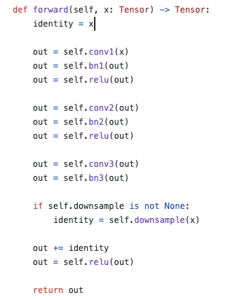
Conv layers are basically the same as our linear layers, but for images, so they have spatial structure. Linear layers process blocks of image data; fully connected layers have no spatial concept.
The basic structure is the same: a weight layer, a normalization layer, and nonlinearity.
Summary (TL;DR)
Understanding activations, gradients, and their statistics in neural networks is vital, especially as networks get larger and deeper.
Review:
Initialization Fix: Overconfident wrong predictions lead to chaotic activations in the final layer and hockey stick losses. Fixing this improves loss by avoiding wasted training.
Weight Initialization: Control activation distributions; you don’t want them squashed to 0 or infinite. You want everything uniform, close to Gaussian. The question is how to scale weight matrices and biases. You can currently look up tables to precisely define them.
Batch Norm: As networks grow deeper, normalization layers are needed. Batch normalization was first. If you want a roughly Gaussian distribution, take mean and std and center the data.
Batch Norm Inference Issues: Moving mean/std estimation into training results in batch norm layers that effectively control activation statistics. However, they introduce bugs, so alternatives like group normalization or layer normalization are preferred.
With advanced optimizers like Adam or Residual connections, training neural networks requires precision at every step, considering initialization, activations, and gradients. Training very deep networks otherwise is impossible.
Supplement 1: Why Tanh is Needed
Why include them and consider their gain?
Simple: with only linear layers, we’d get good activations easily, but the overall network would just be a linear layer. No matter how many you stack, you only get a linear transformation.
Tanh nonlinearity turns this “linear sandwich” into a neural network that can approximate any function.
Supplement 2: Setting the Learning Rate
Andrej Karpathy mentions an empirical method to check if the learning rate is set correctly, involving calculating the ratio of the gradient update to the parameter value itself.
This “ratio” is the ratio of parameter change to the current parameter value in a single update. It’s calculated as the update step (gradient times learning rate) divided by the absolute value of the parameter. For a parameter , gradient , and learning rate $$:
If this ratio is in a reasonable range, say around -3 (on a log scale, i.e., ), the learning rate is neither too large (leading to explosive updates) nor too small (leading to slow, ineffective training). This ensures updates are gentle enough to promote learning without causing instability.
This ratio can monitor and adjust learning rates—reduce if too large, increase if too small. It’s a heuristic to help debug neural network models.