History of LLM Evolution (2): Embeddings — MLPs and Deep Language Connections

The source code repository for this section.

《A Neural Probabilistic Language Model》

This paper is a classic in training language models. Bengio introduced neural networks into language model training and obtained word embeddings as a byproduct. Word embeddings contributed significantly to the subsequent success of deep learning in natural language processing and are an effective way to obtain semantic features of words.

The paper originated to solve the curse of dimensionality caused by original word vectors (one-hot representation). The authors suggested solving this problem by learning a distributed representation for words. Based on the n-gram model, they trained a neural network using a corpus to maximize the prediction of the current word based on the previous $n$ words. The model simultaneously learned the distributed representation of each word and the probability distribution function of word sequences.

Classic formula

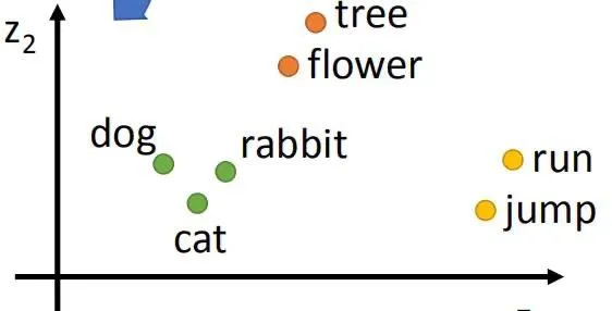
The vocabulary representations learned by this model differ from traditional one-hot representations. Similarity between words can be represented through distances (Euclidean, cosine, etc.) between word embeddings. For example, in “The cat is walking in the bedroom; A dog was running in a room,” ‘cat’ and ‘dog’ have similar semantics. You can transfer knowledge through the embedding space and generalize it to new scenarios.

$index ∈ (0, 16999)$ Shared look-up table Hidden layer size is a hyperparameter Output layer has 17,000 neurons, fully connected to the hidden layer, i.e., logits

In neural networks, the term “logits” usually refers to the output of the last linear layer (i.e., before the activation function). In classification tasks, this linear output is fed into a softmax function to generate a probability distribution. Logits are essentially unnormalized prediction scores reflecting the model’s confidence level for each category.

Why “logits”?

The term comes from logistic regression, where the “logit” function is the inverse of the logistic function. In binary logistic regression, the relationship between output probability $p$ and logit $L$ is:

$L = \log\left(\frac{p}{1 - p}\right)$ $p/(1-p)$ represents the ratio of the probability of an event occurring to it not occurring, called the odds. Advantages of odds over probability: the output range extends to the entire real number range $(-\infty, +\infty)$, the relationship between features and output is linear, and the likelihood function is concise.

Here, $L$ is the logit. In neural networks, even without directly using the logit function, “logits” describes the raw output because it’s similar to logits in logistic regression before the softmax function.

In multi-class problems, logits are usually a vector where each element corresponds to a category’s logit. For example, in handwritten digit recognition (MNIST), the output logits would be a 10-element vector, each corresponding to a digit (0-9) prediction score.

The softmax function converts logits into a probability distribution:

$\text{softmax}(\text{logits})_i = \frac{e^{\text{logits}_i}}{\sum_{j} e^{\text{logits}_j}}$

Here, $e^{\text{logits}_i}$ exponentiates the $i$-th logit to make it positive, and it’s normalized by the sum of all exponentiated logits to obtain a valid probability distribution.

Summary: In neural networks, logits are raw prediction outputs for each category, typically before applying softmax. These scores reflect prediction confidence and are used during training to calculate loss, especially cross-entropy loss.

Building NPLM

Creating the Dataset

# build the dataset
 
block_size = 3 # context length: how many characters do we take to predict the next one
X, Y = [], []
 
for w in words:
    print(w)
    context = [0] * block_size
    for ch in w + '.':
        ix = stoi[ch]
        X.append(context)
        Y.append(ix)
        print(''.join(itos[i] for i in context), '--->', itos[ix])
        context = context[1:] + [ix] # crop and append
    
X = torch.tensor(X)
Y = torch.tensor(Y)

Now we build the neural network using X to predict Y.

Lookup Table

We embed 27 possible characters into a low-dimensional space (the original paper embedded 17,000 words into a 30D space).

C = torch.randn((27,2))
 
F.one_hot(torch.tensor(5), num_classes=27).float() @ C
# (1, 27) @ (27, 2) = (1, 2)

Equivalent to keeping only the 5th row of C.

Hidden Layer

W1 = torch.randn((6, 100)) # Inputs: 3 x 2 = 6, 100 neurons
b1 = torch.randn(100)
 
emb @ W1 + b1 # Desired form

But since emb has shape [228146, 3, 2], how do we combine 3 and 2 into 6?

• torch.cat(tensors, dim, ):

Since block_size can change, we avoid hard-coding and use torch.unbind(tensors, dim, ) to get a tuple of slices:

This method creates new memory. Is there a more efficient way?

• tensor.view():

a = torch.arange(18)
 
a.storage() # 0 1 2 3 4 ... 17

This is efficient. Every tensor has an underlying storage form—the numbers themselves—always a 1D vector. Calling view() merely changes the interpretation attributes of this sequence. No memory change, copying, moving, or creation occurs; the storage remains identical.

The final look:

emb.view(emb.shape[0], 6) @ W1 + b1
# or 
emb.view(-1, 6) @ W1 + b1

Adding non-linear transformation:

h = torch.tanh(emb.view(-1, 6) @ W1 + b1)

Output Layer

# 27 possible output characters
W2 = torch.randn((100, 27)) 
b2 = torch.randn(27)
 
logits = h @ W2 + b2

As in the previous section, obtain counts and probabilities:

counts = logits.exp()
prob = counts / counts.sum(1, keepdim=True)

Negative log likelihood loss:

loss = -prob[torch.arange(Y.shape[0]), Y].log().mean()

Current loss is over 19, our starting point for optimization.

Reorganizing our network:

g = torch.Generator().manual_seed(2147483647)
C = torch.randn((27,2), generator=g)
W1 = torch.randn((6,100), generator=g)
b1 = torch.randn(100, generator=g)
W2 = torch.randn((100,27), generator=g)
b2 = torch.randn(27, generator=g)
parameters = [C, W1, b1, W2, b2]
 
sum(p.nelement() for p in parameters) # 3481
 
# forward pass
emb = C[X] # (228146, 3, 2)
h = torch.tanh(emb.view(-1, 6) @ W1 + b1) # (228146, 100)
logits = h @ W2 + b2 # (228146, 27)

We can use torch’s cross-entropy loss to replace the previous code:

# counts = logits.exp()
# prob = counts / counts.sum(1, keepdim=True) 
# loss = -prob[torch.arange(Y.shape[0]), Y].log().mean()
loss = F.cross_entropy(logits, Y)

The result is exactly the same.

In practice, PyTorch’s implementation is always used because it performs all operations in a fused kernel, avoiding intermediate memory for tensors. It’s simpler, and forward/backward passes are more efficient. Additionally, the educational implementation would overflow to NaN if a count is very large after exp.

How PyTorch handles this: Example: For logits = torch.tensor([1,2,3,4]) and logits = torch.tensor([1,2,3,4]) - 4, while absolute values differ, their relative differences remain the same. Softmax is sensitive to relative differences, not absolute values.

$\text{softmax}(\text{logits})_i = \frac{e^{\text{logits}_i}}{\sum_{j} e^{\text{logits}_j}}$

Subtracting a constant from logits scales each exponent by the same factor. Since the constant is subtracted from every logit, it cancels out in the numerator and denominator, leaving the final probability distribution unchanged. For any logits vector and constant C:

$\frac{e^{\text{logits}_i - C}}{\sum_{j} e^{\text{logits}_j - C}} = \frac{e^{\text{logits}_i} / e^C}{\sum_{j} e^{\text{logits}_j} / e^C} = \frac{e^{\text{logits}_i}}{\sum_{j} e^{\text{logits}_j}}$

PyTorch avoids numerical overflow when calculating e^logits by internally computing the maximum logit and subtracting it.

Training

for p in parameters:
    p.requires_grad_()
    
for _ in range(10): # Large dataset, testing optimization success first
    # forward pass
    emb = C[X] # (228146, 3, 2)
    h = torch.tanh(emb.view(-1, 6) @ W1 + b1) # (228146, 100)
    logits = h @ W2 + b2 # (228146, 27)
    loss = F.cross_entropy(logits, Y)
 
    # backward pass
    for p in parameters:
        p.grad = None
    loss.backward()
 
    # update
    for p in parameters:
        p.data += -0.1 * p.grad 
 
print(loss.item())

Trained on the full dataset, loss only reaches a relatively small value. Output shows some similarity to correct results. Training on a single batch could achieve overfitting, with predictions matching correct results. Fundamentally, loss won’t reach 0 because many characters are possible for ’…’, preventing complete overfitting.

Mini-batch

Since backpropagating through 220,000 data points is slow, computation is massive. In practice, updates and performance measurements are often done on small batches. We randomly select a part of the dataset—a mini-batch—and iterate on these.

for _ in range(1000):
    # mini-batch
    ix = torch.randint(0,X.shape[0],(32,))
 
    # forward pass
    emb = C[X[ix]] # (32, 3, 2)
    h = torch.tanh(emb.view(-1, 6) @ W1 + b1) # (32, 100)
    logits = h @ W2 + b2 # (32, 27)
    loss = F.cross_entropy(logits, Y[ix])

Iteration is now lightning fast.

This doesn’t optimize in the true gradient direction but takes steps based on an approximate gradient, which is very effective in practice.

Learning Rate

lre = torch.linspace(-3, 0, 1000)
lrs = 10**lre # (0.001 - 1)
 
lri = []
lossi = []
 
for i in range(1000):
		'''
		mini-batch, forward and backward pass code 
		'''
		# update
    lr = lrs[i]
    for p in parameters:
        p.data += -lr * p.grad 
		# tracks stats
	lri.append(lre[i])
		lossi.append(loss.item())
 
plt.plot(lri, lossi)

Loss is minimized near lre = -1.0, making the ideal learning rate $10^{-1} = 0.1$.

Now we can confidently choose a learning rate.

	lr = 0.1
    for p in parameters:
        p.data += -lr * p.grad 

After several 10,000-step iterations, loss stabilizes around 2.4. We can then perform learning rate decay, e.g., reducing it by 10x to 0.01 for a few more rounds, resulting in a roughly trained network.

Much lower loss than the bigram model. Does this mean the model is better?

Not necessarily. Increasing parameter count could push loss very close to 0, but sampling would just yield identical examples from the training set. Loss on unseen words might be huge, so that’s not a good model.

This leads to the standard practice: splitting the dataset into three parts: training split, validation (dev) split, and test split.

1. Training Split:

   • Purpose: Train model parameters (weights and biases).
   • Process: The model learns features and patterns, adjusting parameters via backpropagation and gradient descent to minimize loss.

2. Validation (Dev) Split:

   • Purpose: Train (tune) model hyperparameters (learning rate, number of layers, layer sizes, etc.).
   • Process: Performance is evaluated on the validation set during training to adjust and select optimal hyperparameters. This assesses generalization without touching the test set, preventing overfitting.

3. Test Split:

   • Purpose: Evaluate final performance—potential real-world performance.
   • Process: Completely untouched during development. Used only after the model is trained and hyperparameters are tuned on the validation set. Provides an unbiased evaluation on unseen data.

This splitting helps avoid data leakage and overfitting, where a model performs well on training data but poorly on unseen data. This allows for more confident predictions of real-world performance.

Wrapping the dataset construction into a function for splitting:

def build_dataset(words):
	'''
	previous code
	'''
	return X, Y
 
import random
 
random.seed(42)
random.shuffle(words)
n1 = int(0.8 * len(words))
n2 = int(0.9 * len(words))
 
Xtr, Ytr = build_dataset(words[:n1])     # 80% train
Xdev, Ydev = build_dataset(words[n1:n2]) # 10% validation
Xte, Yte = build_dataset(words[n2:])     # 10% test

Data quantities for each part.

Modifying the training section:

ix = torch.randint(0,Xtr.shape[0],(32,))
loss = F.cross_entropy(logits, Ytr[ix])

Training and validation losses are similar, meaning the model isn’t strong enough to overfit. This is underfitting, usually meaning our network capacity is too small.

The simplest fix is increasing hidden layer neurons:

Now over 10,000 parameters, much larger than the original 3,000+.

Optimization looks “thick” due to noise from mini-batch training.

Performance is still limited by:

• Mini-batch size is too small, noise is too high.
• Embedding is problematic; putting too many characters in a 2D space isn’t effectively utilized by the network.

Visualizing current embeddings:

plt.figure(figsize=(8, 8))
plt.scatter(C[:,0].data, C[:,1].data, s=200)
for i in range(C.shape[0]):
    plt.text(C[i,0].item(), C[i,1].item(), itos[i], ha="center", va="center", color="white")
plt.grid('minor')

Training results are visible: g, q, p, and . are treated as distinct vectors, while x, h, b etc. are similar, interchangeable vectors.

Embeddings are likely the network bottleneck.

C = torch.randn((27,10), generator=g)
W1 = torch.randn((30,200), generator=g)
b1 = torch.randn(200, generator=g)
W2 = torch.randn((200,27), generator=g)

Loss is lower, confirming embeddings were a significant factor.

Further optimization strategies:

• Embedding dimensions
• Context length
• Hidden layer neuron count
• Learning rate
• Training duration
• …

Sampling

Finally, sampling to see results:

g = torch.Generator().manual_seed(2147483647 + 10)
 
for _ in range(20):
    out = []
    context = [0] * block_size # initialize with all ...
    while True:
        emb = C[torch.tensor([context])]  # (1, block_size, D)
        h = torch.tanh(emb.view(1, -1) @ W1 + b1)
        logits = h @ W2 + b2
        probs = F.softmax(logits, dim=1)
        ix = torch.multinomial(probs, num_samples=1, generator=g).item()
        context = context[1:] + [ix]
        out.append(ix)
        if ix == 0:
            break
    print(''.join(itos[i] for i in out))

Some progress is visible.

Next, we move to modern models like CNN, GRU, and Transformers.