History of LLM Evolution (1): The Simplicity of Bigram

The source code repository for this section.

Previously, by implementing micrograd, we understood the meaning of gradients and how to optimize. Now we can enter the stage of learning language models and understand how primary language models are designed and modeled.

Evolution of Language Models

• Bigram (One character predicts the next via a count-based lookup table.)
• MLP, following Bengio et al. 2003
• CNN, following DeepMind WaveNet 2016 (in progress…)
• RNN, following Mikolov et al. 2010
• LSTM, following Graves et al. 2014
• GRU, following Kyunghyun Cho et al. 2014
• Transformer, following Vaswani et al. 2017

In this article, we will focus on the Bigram model, an architecture that seems very simple today. It is based on the Markov chain assumption that the occurrence of the next word depends only on the previous word.

Dataset Introduction

Contains 32,033 English names, ranging in length from 2 to 15 characters.

Information in a Name

Taking ‘isabella’, the 4th name in the dataset, as an example, this word contains many examples, such as:

• The character ‘i’ is very likely to appear in the first position of a name.
• ’s’ is likely to follow ‘i’.
• ‘a’ is likely to follow ‘is’… and so on.
• After ‘isabella’ appears, the word is likely to end, which is crucial information.

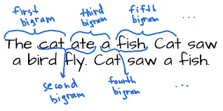
Bigram

In this model, we always process only 2 characters at a time, meaning we only look at one given character to predict the next character in the sequence. It only models this local structure, making it a very simple and weak model.

for w in words[:3]:
    chs = ['<S>'] + list(w) + ['<E>']
    for ch1, ch2 in zip(chs, chs[1:]):
        print(ch1, ch2)

The simplest way to implement a bigram is through “counting,” so we basically just need to count how frequently these combinations appear in the training set.

We can use a dictionary to maintain the count for each bigram:

Creating mapping relationships for character combinations:

N = torch.zeros((28,28), dtype=torch.int32)
 
chars = sorted(list(set(''.join(words))))
stoi = {s:i+1 for i,s in enumerate(chars)}
stoi['.'] = 0 # Replace markers with . to avoid impossible situations like <S> being the second letter
itos = {i:s for s,i in stoi.items()}
itos

Copy and modify the previous count statistics loop:

for w in words:
    chs = ['.'] + list(w) + ['.']
    for ch1, ch2 in zip(chs, chs[1:]):
        ix1 = stoi[ch1]
        ix2 = stoi[ch2]
        N[ix1, ix2] += 1

To make the output more attractive, use the matplotlib library:

import matplotlib.pyplot as plt
%matplotlib inline
 
plt.figure(figsize=(16,16))
plt.imshow(N, cmap='Blues')
for i in range(27):
    for j in range(27):
        chstr = itos[i] + itos[j]
        plt.text(j, i, chstr, ha='center', va='bottom', color='gray')
        plt.text(j, i, N[i, j].item(), ha='center', va='top', color='gray') # N[i,j] is a torch.Tensor, use .item() to get its value
plt.axis('off')

We have now basically completed the sampling required for the Bigram model. Next, we need to sample from the model based on these counts (probabilities):

• Sampling the first character of a name: look at the first row

The counts in the first row tell us the frequency of all characters as the first character.

Now we can use torch.multinomial (a function for random sampling from a given multinomial distribution) to sample from this distribution. Specifically, it randomly draws samples based on weights in an input Tensor, which define the probability of each element being drawn.

For reproducibility, use torch.Generator:

This means: more than half are 0, a small part are 1, and 2 has only a very small quantity.

p = N[0].float()
p = p / p.sum()

The first character is predicted as ‘c’, so next we look at the row starting with ‘c’… and build the loop according to this logic:

Loop 20 times:

for i in range(20):
    out = []
    ix = 0
    while True:
        p = N[ix].float()
        p = p / p.sum()
        ix = torch.multinomial(p, num_samples=1, replacement=True, generator=g).item()
        out.append(itos[ix])
        if ix == 0:
            break
    print(''.join(out))

The results are a bit strange, but the code is fine because this is all the current model design can produce.

The current model might generate single-character names, like ‘h’. The reason is that it only knows the probability of the next character for ‘h’ but doesn’t know if it’s the first character; it only captures very local relationships. However, it’s still better than an untrained model; at least some results look like names.

Currently, the probability is calculated at each iteration. To improve efficiency and practice Tensor operations with the torch API, we use the following:

dim and keepdim=True allow specifying the dimension index. Here, we want to calculate the total for each of the 27 rows separately, which is dim=1 in a 2D tensor.

Additionally, a key point is broadcasting semantics in PyTorch.

In short, if a PyTorch operation supports broadcasting, its tensor arguments can be automatically expanded to the same size (without copying data).

A tensor can be broadcast if:

• Each tensor has at least one dimension.
• When traversing dimension sizes starting from the trailing dimension, they must be equal, or one of them must be 1 or non-existent.

The current situation meets the requirements and is broadcastable, i.e., (27x27) / (27x1). Thus, it’s equivalent to copying (27x1) 27 times and performing division for each row normalization.

P = N.float()
P /= P.sum(dim=1, keepdim=True)
# Use an "in-place operation" to avoid creating a new tensor
 
for i in range(50):
    out = []
    ix = 0
    while True:
        p = P[ix] # Avoid redundant calculation
        ix = torch.multinomial(p, num_samples=1, replacement=True, generator=g).item()
        out.append(itos[ix])
        if ix == 0:
            break
    print(''.join(out))

Final form.

The question then arises: how do we define a loss function to judge how well this model predicts the training set?

Printing the probabilities for each combination, we find that compared to random prediction ($\frac{1}{27} \approx 4\%$), some combinations are as high as 39%. This is clearly a good thing. Especially when your model performs excellently, these expectations should approach 1, meaning the model correctly predicted what happens next in the training set.

Negative Log-Likelihood Loss

So how do we summarize these probabilities into a single number that measures model quality?

When you study literature on maximum likelihood estimation and statistical modeling, you’ll find that something called “likelihood” is typically used. The product of all probabilities in this model is the likelihood, and this product should be as high as possible. The probabilities in the current model are small numbers between 0 and 1, so the overall product will also be a very small value.

For convenience, people usually use “log likelihood.” Here, we just take the logarithm of the probabilities:

Here we change the prob type back to Tensor to call torch.log(). It can be seen that the larger the probability, the closer the log likelihood is to 0.

Plot of $log(x), x \in (0,1)$

Based on basic math: $log(a*b*c) = log(a) + log(b) + log(c)$ Thus, the log likelihood is the sum of the logs of individual probabilities.

Under the current definition, the better the model, the closer the log likelihood value is to 0 and the smaller the error. However, the semantics of a “loss function” is “lower is better,” i.e., “reducing loss.” Therefore, what we need is the opposite of the current expression, which gives us negative log likelihood (NLL):

log_likelihood = 0.0
n = 0 # Count, used for averaging
for w in words[:3]:
    chs = ['.'] + list(w) + ['.']
    for ch1, ch2 in zip(chs, chs[1:]):
        ix1 = stoi[ch1]
        ix2 = stoi[ch2]
        prob = P[ix1, ix2]
        logprob = torch.log(prob)
        log_likelihood += logprob
        n += 1
        print(f'{ch1}{ch2}:{prob:.4f} {logprob:.4f}')
 
nll = -log_likelihood 
print(f'{nll / n}') # normalize

Summary: The current loss function is excellent because its minimum is 0, and a higher value indicates poorer prediction performance. Our training task is to find parameters that minimize the negative log-likelihood loss. Maximizing likelihood is equivalent to maximizing log likelihood because log is a monotonic function, acting as a scaling effect on the original likelihood function. Maximizing log likelihood is equivalent to minimizing negative log likelihood, which in practice becomes minimizing the average negative log likelihood.

Model Smoothing

Take a name containing ‘jq’ as an example. The result obtained here would be: infinite loss. The reason is that ‘jq’ combinations are completely absent from the training set, with a probability of occurrence of 0, leading to this situation:

To solve this, a simple method is model smoothing, where we can add 1 to the count of every combination:

P = (N + 1).float()

The more smoothing added here, the flatter the resulting model; the less added, the more peaked the model will be. 1 is a good value because it ensures that no 0s appear in the probability matrix P, solving the infinite loss problem.

Using a Neural Network Framework

In a neural network framework, the approach to problems will be slightly different, but it will end up in a very similar place. Gradient-based optimization will be used to adjust the parameters of this network, tuning weights so that the neural network can correctly predict the next character.

The first task is to compile the training set for this neural network:

This means that if the input character index is 0, the correctly predicted label should be 5, and so on.

Difference between tensor and Tensor

The difference is that torch.Tensor defaults to float32, whereas torch.tensor automatically infers the data type based on the provided data.

So using the lowercase tensor is recommended. We also want int type integers here, so we use the lowercase version.

One-Hot Encoding

We can’t just plug them in directly because the samples are currently integers representing character indices. Taking an integer index from an input neuron and multiplying it by weights is meaningless.

A common integer encoding method is called one-hot encoding:

Using 13 as an example, in one-hot encoding, we take such an integer and create a vector that is 0 everywhere except for the 13th dimension, which is 1. This vector can be input into a neural network.

import torch.nn.functional as F
 
xenc = F.one_hot(xs, num_classes=27)

Dimension must be specified, otherwise it might guess there are only 13 dimensions.

But now, xenc.dtype shows its type as int64, and torch doesn’t support specifying the output type of one_hot, so a cast is needed:

xenc = F.one_hot(xs, num_classes=27).float()

The result is now a float32 floating-point number, which can be input into a neural network.

Constructing Neurons

As introduced in micrograd, the function a neuron performs is basically $w \cdot x + b$ on input values $x$, where the operation is a dot product:

W = torch.randn((27,27))
# (5,27) @ (27,27) = (5,27)
xenc @ W

Now we have fed 27-dimensional inputs into the first layer of a neural network with 27 neurons.

How do we interpret the neural network’s output?

Our current output has both positive and negative values, while the previous counts and probabilities are positive. So the neural network outputs log counts (denoted as logits). To get positive counts, we take the log counts and then the exponent:

Softmax

# randomly initialize 27 neurons' weights, each neuron receives 27 inputs
g = torch.Generator().manual_seed(2147483647)
W = torch.randn((27,27), generator=g)
 
# Forward pass
 
xenc = F.one_hot(xs, num_classes=27).float()
logits =  xenc @ W # predict log-count
counts = logits.exp() # counts, equivalent to N
probs = counts / counts.sum(dim=1, keepdim=True) # probabilities for next character

btw: the last 2 lines here together are called softmax

Softmax is a layer frequently used in neural networks. It takes log logits, exponentiates, then normalizes them. It’s a method for obtaining outputs from neural network layers where the resulting values always sum to 1 and are all positive, just like a probability distribution. You can place it on top of any linear layer in a neural network.

nlls = torch.zeros(5)
for i in range(5):
    # i-th bigram
    x = xs[i].item()
    y = ys[i].item()
    print('---------')
    print(f'bigram example {i+1}: {itos[x]}{itos[y]} (indexes {x},{y})') 
    print('inputs to neural net:', x)
    print('outputs probabilities from the neural net:', probs[i])
    print('label (actual next character):', y)
    p = probs[i, y]
    print('probability assigned by the net to the correct character:', p.item())
    logp = torch.log(p)
    print(f'logp=')
    nll = -logp
    print('negative log-likelihood:', nll.item())
    nlls[i] = nll
 
print('===========')
print('average negative log-likelihood, i.e. loss:', nlls.mean().item())

The loss is now composed only of differentiable operations. We can adjust $W$ based on the loss gradients for this weight matrix to minimize the loss.

For the first example, these are the probabilities we’re interested in:

To improve the efficiency of accessing these probabilities instead of storing them in tuples like this, you can do the following in torch:

Running backpropagation gives gradient information for each weight:

For example [0,0]=0.0121 means that if this weight increases, its gradient is positive, so the loss will also increase.

Weights can be updated based on this information, analogous to the implementation in micrograd:

W.data += -0.1 * W.grad

Recalculating the forward pass should yield a lower loss:

Indeed, it’s smaller than the previous 3.76.

# gradient descent
for k in range(1000):
 
    # forward pass
    xenc = F.one_hot(xs, num_classes=27).float()
    logits = xenc @ W # predict log-count
    counts = logits.exp() # counts, equivalent to N
    probs = counts / counts.sum(dim=1, keepdim=True) # probabilities for next character
    loss = -probs[torch.arange(5), ys].log().mean() + 0.01 * (W**2).mean() # L2 regularization
    print(loss.item())
 
    # backward pass
    W.grad = None
    loss.backward()
 
    # update
    W.data += -50 * W.grad

Moving forward, as we complexify neural networks all the way to using Transformers, the structure passed into the neural network won’t fundamentally change; only the way we perform the forward pass will change.

Scaling bigrams to more input characters is clearly unrealistic because there would be too many character combinations; the method is not scalable. Neural network methods are significantly more scalable and can be continuously improved, which is the research direction of this course series.

Regularization

It turns out that gradient-based frameworks are equivalent to smoothing: If all elements of $W$ are equal, specifically 0, then logits will become 0. Taking the exponent makes them 1, so the probabilities will be identical.

Therefore, incentivizing W to stay close to 0 is essentially equivalent to label smoothing. The more you incentivize this in the loss function, the smoother the distribution obtained, which leads to “regularization.” We can actually add a small component to the loss function called “regularization loss.”

loss = -probs[torch.arange(5), ys].log().mean() + 0.01 * (W**2).mean() # L2 regularization

Now, besides trying to make all probabilities work, we’re also trying to make all $W$ be 0. Keeping weights close to 0 makes model output less sensitive to input changes, which helps prevent overfitting. In classification tasks, this can lead to more balanced predicted probability distributions across each category, reducing overconfidence in any single category.

Models with the Same Effect

We found that the two models have similar losses, and the sampling results are the same as the model using a probability matrix. They are actually the same model, but the latter approach achieves the same answer with the very different interpretation of a neural network.

Next, we’ll feed more of these types of inputs into neural networks and get the same results. Neural networks output logits, which are still normalized in the same way. All losses and other things in the gradient-based framework remain identical, except the neural network will continue to grow in complexity until it reaches the Transformer.