Introduction to Knowledge Distillation

This article attempts to combine:

• Introductory Demo: Knowledge Distillation Tutorial — PyTorch Tutorials
• Advanced Learning: MIT 6.5940 Fall 2024 TinyML and Efficient Deep Learning Computing, Chapter 9

Knowledge distillation is a technique that enables the transfer of knowledge from large, computationally expensive models to smaller models without losing effectiveness. This allows for deployment on lower-performance hardware, making evaluation faster and more efficient. The process focuses on the outputs rather than just the weights.

Defining Model Classes and Utils

Two different architectures are used, keeping the number of filters constant across experiments for fair comparison. Both architectures are CNNs with different numbers of convolutional layers as feature extractors, followed by a classifier with 10 categories (CIFAR10). The student has fewer filters and parameters.

Teacher Network

Deeper neural network class

class DeepNN(nn.Module):
    def __init__(self, num_classes=10):
        super(DeepNN, self).__init__()
        # 4 convolutional layers, kernels 128, 64, 64, 32
        self.features = nn.Sequential(
            nn.Conv2d(3, 128, kernel_size=3, padding=1),
            nn.ReLU(), # 3 × 3 × 3 × 128 + 128 = 3584
            nn.Conv2d(128, 64, kernel_size=3, padding=1),
            nn.ReLU(), # 3 × 3 × 128 × 64 + 64 = 73792
            nn.MaxPool2d(kernel_size=2, stride=2),
            nn.Conv2d(64, 64, kernel_size=3, padding=1), 
            nn.ReLU(), # 3 × 3 × 64 × 64 + 64 = 36928
            nn.Conv2d(64, 32, kernel_size=3, padding=1),
            nn.ReLU(), # 3 × 3 × 64 × 32 + 32 = 18464
            nn.MaxPool2d(kernel_size=2, stride=2),
        )
        # Output feature map size: 2048, FC layer has 512 neurons
        self.classifier = nn.Sequential(
            nn.Linear(2048, 512), 
            nn.ReLU(), # 2048 × 512 + 512 = 1049088
            nn.Dropout(0.1),
            nn.Linear(512, num_classes) # 512 × 10 + 10 = 5130
        )
 
    def forward(self, x):
        x = self.features(x)
        x = torch.flatten(x, 1)
        x = self.classifier(x)
        return x

Total parameters: 1,177,986

Student Network

Lightweight neural network class

class LightNN(nn.Module):
    def __init__(self, num_classes=10):
        super(LightNN, self).__init__()
        # 2 convolutional layers, kernels: 16, 16
        self.features = nn.Sequential(
            nn.Conv2d(3, 16, kernel_size=3, padding=1),
            nn.ReLU(), # 3 × 3 × 3 × 16 + 16 = 448
            nn.MaxPool2d(kernel_size=2, stride=2),
            nn.Conv2d(16, 16, kernel_size=3, padding=1),
            nn.ReLU(), # 3 × 3 × 16 × 16 + 16 = 2320
            nn.MaxPool2d(kernel_size=2, stride=2),
        )
        # Output feature map size: 1024, FC layer has 256 neurons
        self.classifier = nn.Sequential(
            nn.Linear(1024, 256),
            nn.ReLU(), # 1024 × 256 + 256 = 262400
            nn.Dropout(0.1),
            nn.Linear(256, num_classes) # 256 × 10 + 10 = 2570
        )
 
    def forward(self, x):
        x = self.features(x)
        x = torch.flatten(x, 1)
        x = self.classifier(x)
        return x

Total parameters: 267,738, about 4.4 times fewer than the teacher network.

Training both networks using cross-entropy. The student will serve as a baseline:

def train(model, train_loader, epochs, learning_rate, device):
    criterion = nn.CrossEntropyLoss()
    optimizer = optim.Adam(model.parameters(), lr=learning_rate)
 
    model.train()
 
    for epoch in range(epochs):
        running_loss = 0.0
        for inputs, labels in train_loader:
            # inputs: collection of batch_size images
            # labels: vector of dimension batch_size, integers representing classes
            inputs, labels = inputs.to(device), labels.to(device)
 
            optimizer.zero_grad()
            outputs = model(inputs)
 
            # outputs: network output for the batch, batch_size x num_classes tensor
            # labels: actual labels, batch_size dimension vector
            loss = criterion(outputs, labels)
            loss.backward()
            optimizer.step()
 
            running_loss += loss.item()
 
        print(f"Epoch {epoch+1}/{epochs}, Loss: {running_loss / len(train_loader)}")
 
def test(model, test_loader, device):
    model.to(device)
    model.eval()
 
    correct = 0
    total = 0
 
    with torch.no_grad():
        for inputs, labels in test_loader:
            inputs, labels = inputs.to(device), labels.to(device)
 
            outputs = model(inputs)
            _, predicted = torch.max(outputs.data, 1)
 
            total += labels.size(0)
            correct += (predicted == labels).sum().item()
 
    accuracy = 100 * correct / total
    print(f"Test Accuracy: {accuracy:.2f}%")
    return accuracy

Running Cross-Entropy

torch.manual_seed(42)
nn_deep = DeepNN(num_classes=10).to(device)
train(nn_deep, train_loader, epochs=10, learning_rate=0.001, device=device)
test_accuracy_deep = test(nn_deep, test_loader, device)
# Instantiate student network
torch.manual_seed(42)
nn_light = LightNN(num_classes=10).to(device)

Teacher performance: Test Accuracy: 75.01%

Backpropagation is sensitive to weight initialization, so we need to ensure these two networks have identical initialization.

torch.manual_seed(42)
new_nn_light = LightNN(num_classes=10).to(device)

To verify we’ve created a copy of the first network, we check the norm of its first layer. If they match, the networks are indeed identical.

# Print norm of 1st layer of nn_light
print("Norm of 1st layer of nn_light:", torch.norm(nn_light.features[0].weight).item())
# Print norm of 1st layer of new_nn_light
print("Norm of 1st layer of new_nn_light:", torch.norm(new_nn_light.features[0].weight).item())

Output:

Norm of 1st layer of nn_light: 2.327361822128296 Norm of 1st layer of new_nn_light: 2.327361822128296

total_params_deep = "{:,}".format(sum(p.numel() for p in nn_deep.parameters()))
print(f"DeepNN parameters: {total_params_deep}")
total_params_light = "{:,}".format(sum(p.numel() for p in nn_light.parameters()))
print(f"LightNN parameters: {total_params_light}")

DeepNN parameters: 1,186,986 LightNN parameters: 267,738

Consistent with our manual calculations.

Training and Testing the Student Network with Cross-Entropy Loss

train(nn_light, train_loader, epochs=10, learning_rate=0.001, device=device)
test_accuracy_light_ce = test(nn_light, test_loader, device)

Student performance (without teacher intervention): Test Accuracy: 70.58%

Knowledge Distillation (Soft Targets)

Goal: Matching output logits

Attempting to improve student accuracy by introducing the teacher.

[! Terminology] Knowledge distillation is a technique where, at its most basic, the teacher network’s softmax output is used as an additional loss alongside traditional cross-entropy to train the student. The assumption is that teacher output activations carry extra information that helps the student better learn data similarity structures. Cross-entropy only focuses on the top prediction (activations of unpredicted classes are often tiny), whereas distillation uses the whole output distribution, including smaller probability classes, to more effectively construct an ideal vector space.

Example of similarity structure: in CIFAR-10, if a truck has wheels, it might be mistaken for a car or plane, but is unlikely to be mistaken for a dog.

As seen, the small model’s logits are not confident enough; our motivation is to increase its cat prediction.

Model Mode Setup

Distillation loss is calculated from the network’s logits and only returns gradients for the student. Teacher weights are not updated. We only use its output as guidance.

def train_knowledge_distillation(teacher, student, train_loader, epochs, learning_rate, T, soft_target_loss_weight, ce_loss_weight, device):
    ce_loss = nn.CrossEntropyLoss()
    optimizer = optim.Adam(student.parameters(), lr=learning_rate)
 
    teacher.eval()  # Set teacher to evaluation mode
    student.train() # Set student to training mode
 
    for epoch in range(epochs):
        running_loss = 0.0
        for inputs, labels in train_loader:
            inputs, labels = inputs.to(device), labels.to(device)
 
            optimizer.zero_grad()

Forward Pass and Teacher Output

Using with torch.no_grad() ensures teacher forward pass doesn’t calculate gradients. Saves memory and compute since teacher weights aren’t updated.

            # Forward pass with teacher model
            with torch.no_grad():
                teacher_logits = teacher(inputs)

Student Model Forward Pass

The student model performs a forward pass on the same input, generating student_logits. These logits are used for two losses: soft target loss (distillation loss) and cross-entropy loss with true labels.

            # Forward pass with student model
            student_logits = student(inputs)

Soft Target Loss

• Soft targets are obtained by dividing teacher logits by temperature T and applying softmax. This smooths the teacher’s output distribution.
• Student soft probabilities are calculated by dividing student logits by T and applying log_softmax.

Temperature T > 1 smooths teacher output distribution, helping the student learn more inter-class similarities.

            # Soften student logits by applying log() after softmax
            soft_targets = nn.functional.softmax(teacher_logits / T, dim=-1)
            soft_prob = nn.functional.log_softmax(student_logits / T, dim=-1)

KL Divergence measures the difference between teacher and student output distributions. T**2 is a scaling factor from the “Distilling the knowledge in a neural network” paper used to balance the impact of soft targets.

This loss measures the difference between student and teacher predictions. Minimizing this pushes the student to better mimic the teacher’s representation.

            # Calculate soft target loss
            soft_targets_loss = torch.sum(soft_targets * (soft_targets.log() - soft_prob)) / soft_prob.size()[0] * (T**2)

True Label Loss (Cross-Entropy Loss)

            # Calculate true label loss
            label_loss = ce_loss(student_logits, labels)

• Standard cross-entropy loss evaluates student output against true labels.
• This pushes the student to correctly classify data.

Weighted Total Loss

Total loss is a weighted sum of soft target loss and true label loss. soft_target_loss_weight and ce_loss_weight control the respective weights.

            # Weighted sum of two losses
            loss = soft_target_loss_weight * soft_targets_loss + ce_loss_weight * label_loss

Here soft_target_loss_weight is 0.25 and ce_loss_weight is 0.75, giving true label loss more weight.

Backpropagation and Weight Update

Gradients of the loss with respect to student weights are computed via backpropagation, and the Adam optimizer updates the student weights. This process gradually optimizes student performance by minimizing the loss.

            loss.backward()
            optimizer.step()
 
            running_loss += loss.item()
 
        print(f"Epoch {epoch+1}/{epochs}, Loss: {running_loss / len(train_loader)}")

After training, student performance is evaluated by testing accuracy under different conditions.

# Set T=2, CE weight 0.75, distillation weight 0.25.
train_knowledge_distillation(teacher=nn_deep, student=new_nn_light, train_loader=train_loader, epochs=10, learning_rate=0.001, T=2, soft_target_loss_weight=0.25, ce_loss_weight=0.75, device=device)
test_accuracy_light_ce_and_kd = test(new_nn_light, test_loader, device)
 
# Compare student accuracy with and without teacher guidance
print(f"Teacher accuracy: {test_accuracy_deep:.2f}%")
print(f"Student accuracy without teacher: {test_accuracy_light_ce:.2f}%")
print(f"Student accuracy with CE + KD: {test_accuracy_light_ce_and_kd:.2f}%")

Knowledge Distillation (Hidden Layer Feature Maps)

Goal: Matching intermediate features

Knowledge distillation can extend beyond output layer soft targets to distilling hidden representations of feature extraction layers. Our goal is to transfer teacher representation information to the student using a simple loss function that minimizes the difference between flattened vectors passed to the classifier. Teacher weights remain frozen; only student weights are updated.

The principle assumes the teacher has better internal representations, which the student is unlikely to achieve without intervention, so we push the student to mimic the teacher’s internal representation. However, this isn’t guaranteed to benefit the student since a lightweight network might struggle to reach teacher representations, and learning capacities differ across architectures. In other words, there’s no inherent reason for student and teacher component-wise matches; a student might achieve a permutation of teacher representations. Still, we can experiment using CosineEmbeddingLoss:

Hidden Layer Representation Mismatch

• Teachers are usually more complex with more neurons and higher-dimensional representations. Consequently, flattened convolutional hidden representations often differ in dimension.
• Problem: To use teacher hidden outputs for distillation loss (like CosineEmbeddingLoss), we must ensure matching dimensions.

Solution: Applying Pooling Layers

• Since teacher hidden representations are typically higher-dimensional than student ones after flattening, average pooling is used to reduce teacher output dimensions to match the student’s.
• Specifically, the avg_pool1d function reduces teacher hidden representation dimensions to match the student’s.

def forward(self, x):
    x = self.features(x)
    flattened_conv_output = torch.flatten(x, 1)
    x = self.classifier(flattened_conv_output)
    # Align feature representations
    flattened_conv_output_after_pooling = torch.nn.functional.avg_pool1d(flattened_conv_output, 2)
    return x, flattened_conv_output_after_pooling

Cosine similarity loss is added. By calculating the cosine similarity loss between teacher and student intermediate features, the goal is to bring student feature representations closer to the teacher’s.

cosine_loss = nn.CosineEmbeddingLoss()
hidden_rep_loss = cosine_loss(student_hidden_representation, teacher_hidden_representation, target=torch.ones(inputs.size(0)).to(device))

Since ModifiedDeepNNCosine and ModifiedLightNNCosine return two values (logits and hidden representation), both must be extracted and handled during training.

with torch.no_grad():
    _, teacher_hidden_representation = teacher(inputs)
 
student_logits, student_hidden_representation = student(inputs)

The total loss is a weighted sum of cosine loss and cross-entropy classification loss, controlled by hidden_rep_loss_weight and ce_loss_weight. The final loss consists of classification error (cross-entropy) and similarity between intermediate feature layers (cosine loss).

loss = hidden_rep_loss_weight * hidden_rep_loss + ce_loss_weight * label_loss

Regressor Network

Simple minimization doesn’t guarantee better results due to high vector dimensions, difficulty in extracting meaningful similarities, and a lack of theoretical support for matching hidden representations. We introduce a regressor network to extract and match feature maps after convolutional layers. The regressor is trainable, optimizing the matching process and providing a teaching path for backpropagation gradients to change student weights.

Feature Map Extraction

In ModifiedDeepNNRegressor, the forward pass returns both classifier logits and intermediate conv_feature_map from the feature extractor. This allows for distillation using these maps, comparing student feature maps to teacher ones to enhance performance.

conv_feature_map = x
 
return x, conv_feature_map

Distillation thus extends beyond final logits to internal intermediate representations. This method is expected to outperform CosineLoss because the trainable regressor layer provides flexibility for the student instead of forcing direct copying. Including an extra network is the core idea behind hint-based distillation.

Knowledge Distillation (Extensions)

Weight matching is also possible:

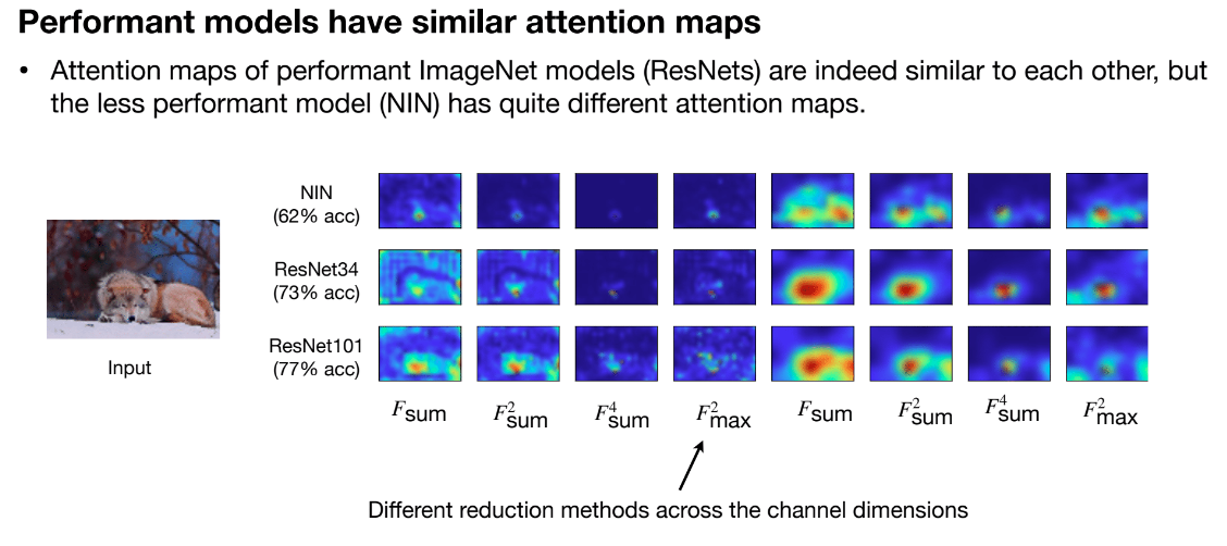
• Gradients: Such as Attention Maps in Transformers, representing input parts the model focuses on. Matching these helps the student learn the teacher’s attention mechanisms.

• Sparsity Patterns: Teachers and students should have similar sparsity patterns after ReLU activation. A neuron is active if its value $> 0$ after ReLU. Use indicator function $\rho(x) = \mathbf{1}[x > 0]$ to represent activation. Matching these patterns helps the student learn the weight or activation sparsity structure, improving efficiency and generalization.

• Relational Information:

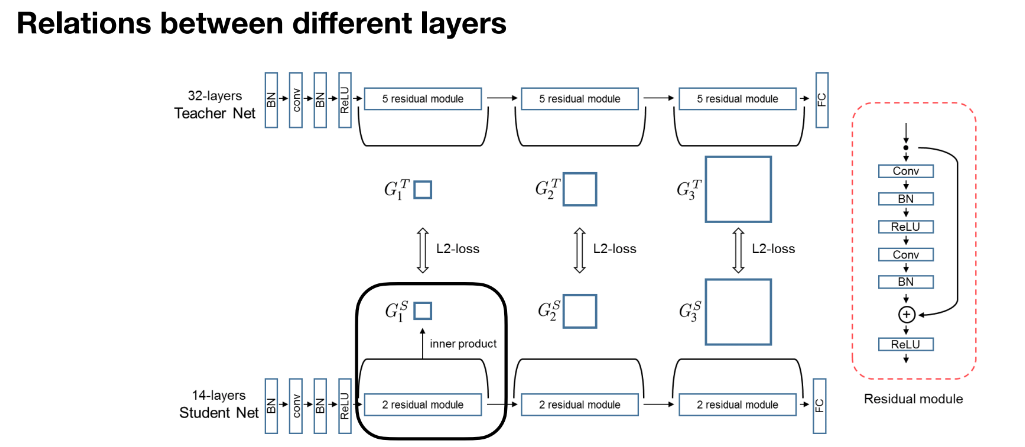
  Calculate relations between layers using inner products. Layer outputs are represented as matrices, and inter-layer relations are matched. L2 loss aligns these relations so feature distributions across layers match.

Traditional distillation matches features or logits for a single sample, whereas Relational Knowledge Distillation focuses on relations across multiple samples. Comparing these relations across teacher and student models helps build structure among samples. This method focuses on associations between multiple input samples rather than point-to-point matching for a single sample.

The method further calculates pairwise distances between samples for both student and teacher networks, using this relational information for distillation. By constructing feature vector distance matrices for sample sets, structural information is transferred to the student. Unlike individual distillation, this method transfers structural relationships across multiple samples.