Ditching the SDEs: A Simpler Path with Flow Matching

This post mainly follows the teaching structure of the video above, with my own re-organization and explanations mixed in. If you spot mistakes, feel free to point them out in the comments!

Flow Matching: Rebuilding Generative Models from First Principles

Alright, let’s talk about generative models. The goal is simple, right? We have a dataset—say, a bunch of cat images—drawn from some wild, high-dimensional distribution $p_1(x_1)$. We want to train a model that can spit out brand-new cat images. The goal is simple, but the method can get… well, pretty gnarly.

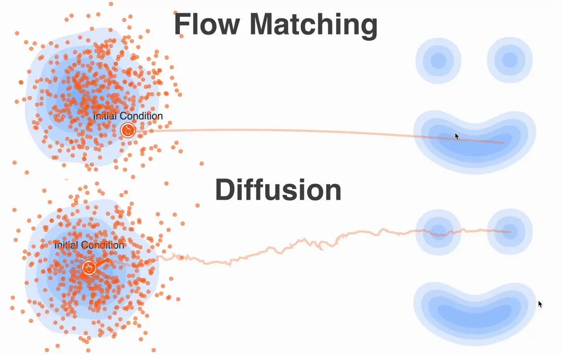
You’ve probably heard of diffusion models. The idea is to start from an image, add noise step by step over hundreds of steps, then train a big network to reverse that process. The math involves score functions ($\nabla_x \log p_t(x)$), stochastic differential equations (stochastic differential equations, SDEs)… it’s a whole thing. It works—and works surprisingly well—but as a computer scientist I always wonder: can we reach the same goal in a simpler, more direct way? Is there a way to hack it?

Let’s step back and start from scratch. First principles.

The Core Problem

We have two distributions:

1. $p_0(x_0)$: a super simple noise distribution we can sample from easily. Think x0 = torch.randn_like(image).
2. $p_1(x_1)$: the real data distribution—complex and unknown (cats!). We can sample from it by loading an image from the dataset.

We want to learn a mapping that takes a sample from $p_0$ and transforms it into a sample from $p_1$.

The diffusion approach defines a complicated distribution path $p_t(x)$ that gradually morphs $p_1$ into $p_0$, then learns how to reverse it. But that intermediate distribution $p_t(x)$ is exactly where the mathematical complexity comes from.

So what’s the simplest thing we could possibly do?

A Naive “High-School Physics” Idea

What if we just… draw a straight line?

Seriously. Pick a noise sample $x_0$ and a real cat image sample $x_1$. What’s the simplest path between them? Linear interpolation.

Here $t$ is our “time” parameter, going from $0$ to $1$.

• When $t=0$, we’re at noise $x_0$.
• When $t=1$, we’re at the cat image $x_1$.
• For any $t$ in between, we’re at some blurry mixture of the two.

Now, imagine a particle moving along this straight-line path from $x_0$ to $x_1$ in one second. What’s its velocity? Let’s stick to high-school physics and differentiate with respect to time $t$:

Hold on. Let that result sit in your head for a moment.

Along this simple straight-line path, the particle’s velocity at any time is just a constant vector pointing from start to end. That’s the simplest vector field you can imagine.

That’s the “Aha!” moment. What if this is all we need?

Building the Model

Now we have a target: we want to learn a vector field. Let’s define a neural network $v_\theta(x, t)$ that takes any point $x$ and any time $t$ as input, and outputs a vector—its predicted velocity at that point.

How do we train it? We want the network output to match our simple target velocity $x_1 - x_0$. The most direct choice is Mean Squared Error.

So the training objective becomes:

Let’s break down the training loop. It’s almost comically simple:

x1 = sample_from_dataset()        # grab a real cat image
x0 = torch.randn_like(x1)         # sample some noise
t = torch.rand(1)                 # pick a random time
xt = (1 - t) * x0 + t * x1        # interpolate to get the training input point
predicted_velocity = model(xt, t) # ask the model to predict the velocity
target_velocity = x1 - x0         # this is our ground truth!
loss = mse_loss(predicted_velocity, target_velocity)
loss.backward()
optimizer.step()

Boom. That’s it. This is the core of Conditional Flow Matching. We turned a puzzling distribution-matching problem into a simple regression problem.

Why This Is So Powerful: “Simulation-Free”

Notice what we didn’t do. We never had to mention the complicated marginal distribution $p_t(x)$. We never had to define or estimate a score function. We bypass the entire SDE/PDE machinery.

All we need is the ability to sample pairs $(x_0, x_1)$ and interpolate between them. That’s why it’s called simulation-free training. It’s unbelievably direct.

Generating Images (Inference)

Now we’ve trained $v_\theta(x, t)$—a great “GPS” that can navigate from noise to data. How do we generate a new cat image?

We just follow its directions:

1. Start from random noise: x = torch.randn(...).
2. Start at time $t=0$.
3. Iterate for a number of steps: a. Get a direction from our “GPS”: velocity = model(x, t). b. Take a small step: x = x + velocity * dt. c. Update time: t = t + dt.
4. After enough steps (e.g., when $t$ reaches 1), x becomes our new cat image.

This is just solving an ordinary differential equation (Ordinary Differential Equation, ODE). It’s basically Euler’s method—something you might’ve even seen in high school. Pretty cool, right?

Summary

So to recap: Flow Matching gives us a fresh, simpler way to think about generative modeling. Instead of thinking in terms of densities and scores, we think in terms of vector fields and flows. We define a simple path from noise to data (like a straight line), then train a neural network to learn the velocity field that generates that path.

It turns out this simple, intuitive idea isn’t just a hack: it’s theoretically sound, and it powers some recent state-of-the-art models like SD3. It’s a great reminder that sometimes the deepest progress comes from finding a cleaner abstraction for a complex problem.

Simplicity wins.

The “Proper” Derivation: Why Does Our Simple “Hack” Work?

So far we derived Flow Matching’s core with an extremely simple intuition: take a noise sample $x_0$, a data sample $x_1$, draw a straight line between them ($x_t = (1-t)x_0 + t x_1$), and say the network $v_\theta$ only needs to learn the velocity—i.e., $x_1 - x_0$. The loss almost writes itself. Done.

Honestly, for most practitioners, that’s 90% of what you need.

But if you’re like me, a little voice might whisper: “Wait… this feels too easy. Our trick is built on a pair of independent samples $(x_0, x_1)$. Why should learning these independent straight lines make the network understand the flow of the entire high-dimensional probability distribution $p_t(x)$? Is this a legit shortcut, or a lucky, slightly cute hack that just happens to work?”

That’s where the formal derivation in the paper comes in. Its job is to show that our simple conditional objective can indeed (almost magically) optimize the bigger, scarier marginal objective.

Let’s put on a mathematician’s hat for a moment and see how they bridge the gap.

The “Official” Theoretical Problem: Marginal Flows

The “real” theoretical setup is: we have a family of distributions $p_t(x)$ that continuously morphs from noise $p_0(x)$ to data $p_1(x)$. This continuous deformation is governed by a vector field $u_t(x)$—the velocity at time $t$ and position $x$.

So the “official” goal is to train $v_\theta(x, t)$ to match the true marginal vector field $u_t(x)$. The loss would be:

And this is immediately a disaster: it’s intractable. We can’t sample from $p_t(x)$, and we don’t know the target $u_t(x)$. So in this form, the loss is useless.

The Bridge: Connecting “Marginal” and “Conditional”

Researchers use a classic trick: “Sure, the marginal field $u_t(x)$ is a beast. But can we express it as an average over simpler conditional vector fields?”

A conditional vector field $u_t(x|x_1)$ is the velocity at point $x$ given that we already know the final destination is the data point $x_1$.

The paper proves (and this is the key theoretical insight) that the scary marginal field $u_t(x)$ is the expectation over these simple conditional fields, weighted by “the probability that a path starting from $x_1$ passes through $x$”:

This builds the bridge: we relate an unknown quantity ($u_t(x)$) to many simpler things we might be able to define ($u_t(x|x_1)$).

We start from the “official” marginal flow matching loss. For any fixed time $t$, it is:

Here $p_t(x)$ is the marginal density at time $t$, and $u_t(x)$ is the true marginal vector field we want to learn. We can’t access either, so this form can’t be computed. The goal is to transform it into something computable.

Step 1: Expand the squared error

Using the identity $\|A - B\|^2 = \|A\|^2 - 2A \cdot B + \|B\|^2$:

During optimization we only care about terms that depend on $\theta$. The term $\|u_t(x)\|^2$ does not depend on $\theta$, so it can be treated as a constant for gradients. To minimize $L_t(v_\theta)$, it’s enough to minimize:

Step 2: Rewrite the expectation as an integral

Using $\mathbb{E}_{x \sim p(x)}[f(x)] = \int p(x)f(x)dx$, and focusing on the cross term with the unknown $u_t(x)$:

Step 3: Substitute the bridge identity

The key identity links the hard marginal term $p_t(x) u_t(x)$ to conditional terms:

Substitute into the cross term:

Step 4: Swap integration order (Fubini–Tonelli theorem)

We now have a double integral. It looks more complex, but we can swap the order of $dx$ and $dx_1$:

Step 5: Convert integrals back to expectations and complete the square

The inner part $\int p_t(x|x_1) v_\theta(x,t) \cdot u_t(x|x_1) dx$ is an expectation over $p_t(x|x_1)$, so:

And since this is also an integral over $p_1(x_1)$, we can write it as an expectation over $x_1$:

This nested expectation can be merged into an expectation over the joint distribution:

Now substitute this back into $L_t'(v_\theta)$. With a similar transformation, the first term becomes $\mathbb{E}_{x_1, x \sim p_t(\cdot|x_1)} [ \|v_\theta(x,t)\|^2 ]$. So:

To form a perfect square, add and subtract the same term $\mathbb{E}_{x_1, x \sim p_t(\cdot|x_1)} \left[ \|u_t(x|x_1)\|^2 \right]$:

The bracketed part is a complete square. The final subtracted term doesn’t depend on $\theta$, so we can ignore it during optimization.

Final result

We’ve shown that minimizing the original intractable marginal loss is equivalent to minimizing the following Conditional Flow Matching Objective:

So we have a rigorous justification: if we define a simple conditional path (like linear interpolation) and its vector field, and optimize this simple regression loss, we still achieve the grand goal of optimizing the true marginal flow.

This is huge: we eliminated the dependence on the marginal density $p_t(x)$. The loss now depends only on the conditional path density $p_t(\cdot|x_1)$ and the conditional vector field $u_t(x|x_1)$.

Back to Our Original Simple Idea

Where does that leave us? The formal proof says: as long as we can define a conditional path $p_t(x|x_1)$ and its corresponding vector field $u_t(x|x_1)$, we can train with $L_{FM}$.

Now we can invite the “high-school physics” idea back in. Since we’re free to define the conditional path, let’s pick the simplest, least pretentious option:

1. Define the conditional path $p_t(\cdot|x_0, x_1)$: make it deterministic—a straight line. So the probability is 1 on the line $x_t = (1-t)x_0 + t x_1$ and 0 everywhere else. (In diffusion, paths from $x_0$ are stochastic.)
2. Define the conditional vector field $u_t(x_t|x_0, x_1)$: as we computed earlier, the velocity is $x_1 - x_0$.

[!NOTE] In math, this kind of “all mass at a single point, zero elsewhere” distribution is called the Dirac delta function $\delta$. So when we choose a straight-line path, we’re effectively choosing a Dirac delta distribution for $p_t(x|x_0, x_1)$.

Now plug these into the fancy-looking $L_{FM}$ objective we derived. The expectation $\mathbb{E}_{x \sim p_t(\cdot|x_1)}$ becomes “take the point $x_t$ on our line”, and the target $u_t(x|x_1)$ becomes the simple $x_1 - x_0$.

And then—the magic moment—we end up with:

We’re back at the exact same ultra-clean loss we “guessed” from first principles. That’s what the formal derivation is for.

Summary

Pretty cool. We just went through a bunch of heavy math—integrals, Fubini’s theorem, the whole package—just to prove that our simple intuitive shortcut was correct from the start. We’ve confirmed: learning the simple vector target $x_1 - x_0$ along a straight-line path is a valid way to train a generative model.

From Theory to torch: Coding Flow Matching

Now that we’ve got the intuition (and even the full formal proof), we can remember: this is still just a regression problem. So let’s look at code.

Surprisingly, the PyTorch implementation is almost a 1:1 translation of the final formula. No hidden complexity, no scary math libraries—just pure torch.

Let’s break down the most important parts: the training loop and the sampling (inference) process.

Source code from the video: https://github.com/dome272/Flow-Matching/blob/main/flow-matching.ipynb

Setup: Data and Model

First, the script sets up a 2D checkerboard pattern. This is our tiny “cat image dataset”. These points are our real data $x_1$.

Then it defines a simple MLP (multilayer perceptron). This is our neural network—our “GPS”, our vector-field predictor $v_\theta(x,t)$. It’s a standard network that takes a batch of coordinates x and a batch of times t, and outputs a predicted velocity vector for each point. Nothing fancy in the architecture—the magic is in what we ask it to learn.

Training Loop: Where the Magic Happens

This is the core. Let’s recall the final, beautiful loss:

Now let’s walk through the training loop line by line. This is the formula in action.

data = torch.Tensor(sampled_points)
training_steps = 100_000
batch_size = 64
pbar = tqdm.tqdm(range(training_steps))
losses = []
 
for i in pbar:
	# 1. Sample real data x1 and noise x0
    x1 = data[torch.randint(data.size(0), (batch_size,))]
    x0 = torch.randn_like(x1)
    
    # 2. Define the target vector
    target = x1 - x0
    
    # 3. Sample random time t and create the interpolated input xt
    t = torch.rand(x1.size(0))
    xt = (1 - t[:, None]) * x0 + t[:, None] * x1
    
    # 4. Get the model's prediction
    pred = model(xt, t)  # also add t here
    
    # 5. Calculate the loss and other standard boilerplate
    loss = ((target - pred)**2).mean()
    loss.backward()
    optim.step()
    optim.zero_grad()
    pbar.set_postfix(loss=loss.item())
    losses.append(loss.item())

Mapping directly to the formula:

• x1 = ... and x0 = ...: sample from the data distribution $p_1$ and the noise distribution $p_0$ to supply $x_1$ and $x_0$ for the expectation $\mathbb{E}$.

• target = x1 - x0: this is the heart of it. This line computes the true vector field for our straight-line path—i.e. the target $\color{red}{(x_1 - x_0)}$.

• xt = (1 - t[:, None]) * x0 + t[:, None] * x1: this is the other key part. It computes the interpolated point $x_t$ on the path—the model input $\color{blue}{(1-t)x_0 + tx_1}$.

• pred = model(xt, t): forward pass to get the prediction $v_\theta(x_t,t)$.

• loss = ((target - pred)**2).mean(): mean squared error between target and prediction—the $\|\cdot\|^2$ part.

That’s it. These five lines are a direct line-by-line implementation of the elegant formula we derived.

Sampling: Following the Flow 🗺️

Now we’ve trained the model. It’s a highly skilled “GPS” that knows the velocity field. How do we generate new checkerboard samples? Start from empty space (noise), and walk where it tells you to go.

Mathematically, we want to solve the ODE: $\frac{dx_t}{dt} = v_\theta(x_t, t)$ The simplest way to solve it is Euler’s method: take small discrete steps to approximate continuous flow.

[!TIP] Since $v_\theta$ is a complex neural network, we can’t solve this analytically. We must simulate it. The simplest approach is to approximate smooth continuous flow with a sequence of small straight-line steps.

By the definition of the derivative, over a small time step $dt$, the position change $dx_t$ is approximately velocity times the time step: $dx_t \approx v_\theta(x_t, t) \cdot dt$.

So to get the new position at $t + dt$, we add this small change to the current position. This gives the update rule:

$x_{t+dt} = x_t + v_\theta(x_t, t) \cdot dt$

This “move a tiny bit along the velocity direction” has a famous name: Euler’s method (Euler update). It’s the simplest numerical solver for ODEs—and as you can see, it almost falls out of first principles.

# The sampling loop from the script
xt = torch.randn(1000, 2)  # Start with pure noise at t=0
steps = 1000
for i, t in enumerate(torch.linspace(0, 1, steps), start=1):
    pred = model(xt, t.expand(xt.size(0))) # Get velocity prediction
    
    # This is the Euler method step!
    # dt = 1 / steps
    xt = xt + (1 / steps) * pred

• xt = torch.randn(...): start from a random point cloud—our initial state.

• for t in torch.linspace(0, 1, steps): simulate flow from $t=0$ to $t=1$ over discrete steps.

• pred = model(xt, ...): at each step, query the current velocity $v_\theta(x_t, t)$.

• xt = xt + (1 / steps) * pred: Euler update. Move xt a tiny step in the predicted direction. Here dt = 1 / steps.

Repeat this update, and the random point cloud gradually gets “pushed” by the learned vector field until it flows into the checkerboard data distribution.

Theoretical simplicity translates directly into clean, efficient code. It’s genuinely beautiful.

DiffusionFlow

But wait… before we celebrate, let’s pause for a “thought bubble” moment.

[!WARNING] The math above works under the assumption that we use a straight-line path between $x_0$ (random noise) and $x_1$ (a random cat image). But… is a straight line really the best, most efficient path?

From a chaotic Gaussian noise cloud to the delicate high-dimensional manifold where real images live, the “true” transformation is likely a wild, winding journey. Forcing a straight line might be too crude. We ask a single neural network $v_\theta$ to learn a vector field that magically works for all these unnatural linear interpolations. This may be one reason we still need many sampling steps for high-quality images: the learned vector field has to keep correcting for our oversimplified path assumption.

So a good “hacker” would naturally ask next: “Can we make the learning problem easier?”

Imagine… instead of pairing completely random $x_0$ and $x_1$, we could find “better” start/end points—say a pair $(z_0, z_1)$ that are naturally related, so the path between them is already close to a straight line.

Where do such pairs come from? Simple: use another generative model (e.g. a standard DDPM) to generate them. Give it a noise vector $z_0$; after hundreds of steps it outputs a decent image $z_1$. Now we have a pair $(z_0, z_1)$ that represents the “real” trajectory taken by a strong model.

This gives us a teacher–student framework: the old, slow model provides these “pre-straightened” trajectories, and we use them to train a new, simpler Flow Matching model. The new model’s learning problem becomes much easier.

This idea—using one model to construct an easier learning problem for another—is powerful. You’re essentially “distilling” a complex, curved path into a simpler, straighter one. Teams at DeepMind and elsewhere had the same idea: it’s the core of Rectified Flow / DiffusionFlow—iteratively straightening the path until it’s so straight you can almost jump from start to end in one step.

It’s a beautiful meta-level extension of our original shortcut. Worth savoring.

References