The Way of Fine-Tuning

Why Fine-Tuning?

When choosing an LLM to complete an NLP task, where do you start? The following diagram clearly illustrates which operation is suitable for your current task:

If you have time and a massive amount of data, you can completely retrain a model. With a moderate amount of data, you can fine-tune a pre-trained model. If you don’t have much data, the best choice is “in-context learning,” such as RAG.

Of course, we are primarily focusing on the fine-tuning part here. Fine-tuning allows us to achieve better performance than the original model without having to retrain it from scratch.

How to Fine-Tune?

As is well known, the graphics card (VRAM) is the bottleneck for casual players trying to use LLMs. Most people only have access to consumer-grade cards, like the RTX series. Therefore, we need to find a smart way to fine-tune using 16GB of VRAM.

Bottlenecks in Fine-Tuning

When training a model with a moderate number of parameters, such as Llama 7B, we might need roughly 28GB of VRAM to store the model’s original parameters (I’ll explain how this is estimated below), an equal amount of VRAM for gradients during training, and typically twice that amount to track the optimizer states.

Let’s do the math:

So, who is going to give me the 96GB of VRAM I’m missing?

Solving the Problem

Half-Precision

The first step is loading the model itself. For a 7B model, each parameter is a 32-bit floating-point number. One byte is 8 bits, so 32 bits require 4 bytes (4B). 7 Billion, or 7,000,000,000, requires a total storage size of $7,000,000,000 \times 4B = 28,000,000,000B \approx 28GB$. ($1GB = 2^{10}MB = 2^{10} \times 2^{10}KB = 2^{30}B = 1,073,741,824B$)

We are over by 28 - 16 = 12GB here. Therefore, we need to find a way to pack model parameters into a smaller form. A very natural idea is to target the parameter units: can we switch to 16 or 8-bit floating-point numbers? (corresponding to 2B and 1B units of storage respectively). Simply switching to FP16 would halve the VRAM requirement for this part. As a tradeoff, the corresponding floating-point precision and representation range will decrease, potentially leading to gradient explosion or disappearance. Google proposed bfloat16 (brain float) for this purpose. Its core goal is to provide a floating-point format that maintains a wide numerical range (compared to IEEE standards, exponent: 5 bits to 8 bits) while simplifying hardware implementation (fraction: 10 bits to 7 bits), thereby accelerating the training and inference of deep learning models without sacrificing too much precision.

By choosing 16-bit floating-point numbers, the VRAM requirement is halved, and one card becomes enough:

Quantization

Let’s briefly describe the neural network training workflow:

We perform a forward pass on the input (activation), then compare the results with predicted targets. Based on the difference between the prediction and the actual target (loss), we calculate the gradient (partial derivative) of the loss function for each parameter for backpropagation (BP). We select an optimization algorithm (like SGD, stochastic gradient descent) to update parameters, and after multiple iterations, we obtain the model.

Gradients in a model usually have the same data type as the original parameters. Since every parameter has a corresponding gradient, we need double the VRAM of the parameters even before considering the optimizer.

Usually, a Quantization method is used, and we can choose 8-bit floating-point numbers.

Image from Nvidia Blog

During the quantization process, the representation range of data is compressed. Data becomes more concentrated, and differences between parameters decrease, which can lead to significant information loss. Clipping outliers that fall outside the new representation range can reduce quantization errors caused by these extreme values.

By choosing int8 quantization, we cut the memory needed for model parameters and gradients to 14GB:

LoRA

Despite these efforts, the optimizer remains a critical part.

The industry-favored Adam optimizer works well but has quite a high memory footprint for the following reasons:

The Adam optimizer updates parameters $\theta$ at each iteration using the following update formula (no need to dive deep into the math):

1. Calculate the first moment estimate (mean of the gradient) and the second moment estimate (uncentered variance of the gradient):

$m_t = \beta_1 \cdot m_{t-1} + (1 - \beta_1) \cdot g_t$

$v_t = \beta_2 \cdot v_{t-1} + (1 - \beta_2) \cdot g_t^2$

Where $g_t$ is the gradient at timestep $t$, $\beta_1$ and $\beta_2$ are decay rates usually close to 1, corresponding to the exponential moving average introduced in section 3 of Karpathy’s Batch-Norm tutorial.

2. Perform bias correction on $m_t$ and $v_t$ to correct their initialization bias towards 0:

$\hat{m}_t = \frac{m_t}{1 - \beta_1^t}$

$\hat{v}_t = \frac{v_t}{1 - \beta_2^t}$

3. Update parameters using the corrected first and second moment estimates:

$\theta_{t+1} = \theta_t - \frac{\eta}{\sqrt{\hat{v}_t} + \epsilon} \cdot \hat{m}_t$

Where $\eta$ is the learning rate and $\epsilon$ is a tiny constant added for numerical stability.

This process repeats at each timestep until parameters converge or a stopping condition is met.

For the momentum vector and variance vector in step 1, each has 7B parameters. This is why we need twice the parameter count as mentioned earlier.

The solution here is LoRA (Low-Rank Adaptation):

This technique reduces the number of trainable parameters, achieving a smaller model weight footprint and faster training. In this scenario, LoRA significantly reduces the number of parameters tracked by the optimizer and gradients, reducing the VRAM required during training.

The key idea behind LoRA is that when fine-tuning a large model like Llama 2, you don’t need to fine-tune every parameter (full parameter fine-tuning). Usually, some parameters and layers are more important than others, such as those responsible for attention mechanisms and determining which tokens in a sequence relate to others and how. LoRA takes these specific parameters and injects low-rank matrices. During training, backpropagation, and parameter updates, only these auxiliary low-rank matrices are modified.

The Rank hyperparameter R in LoRA can be adjusted. Generally, in practice, LoRA might only target less than 10% of the total parameters.

For LoRA parameters, a higher precision fp16 is chosen, while optimizer states are in fp32 units, meaning the memory footprint is four times the number of parameters here.

However, there’s another issue: activation. The overhead during the forward pass of activation is the size of the largest layer in the neural network multiplied by the batch size. This could still take up 5GB of memory, exceeding our budget.

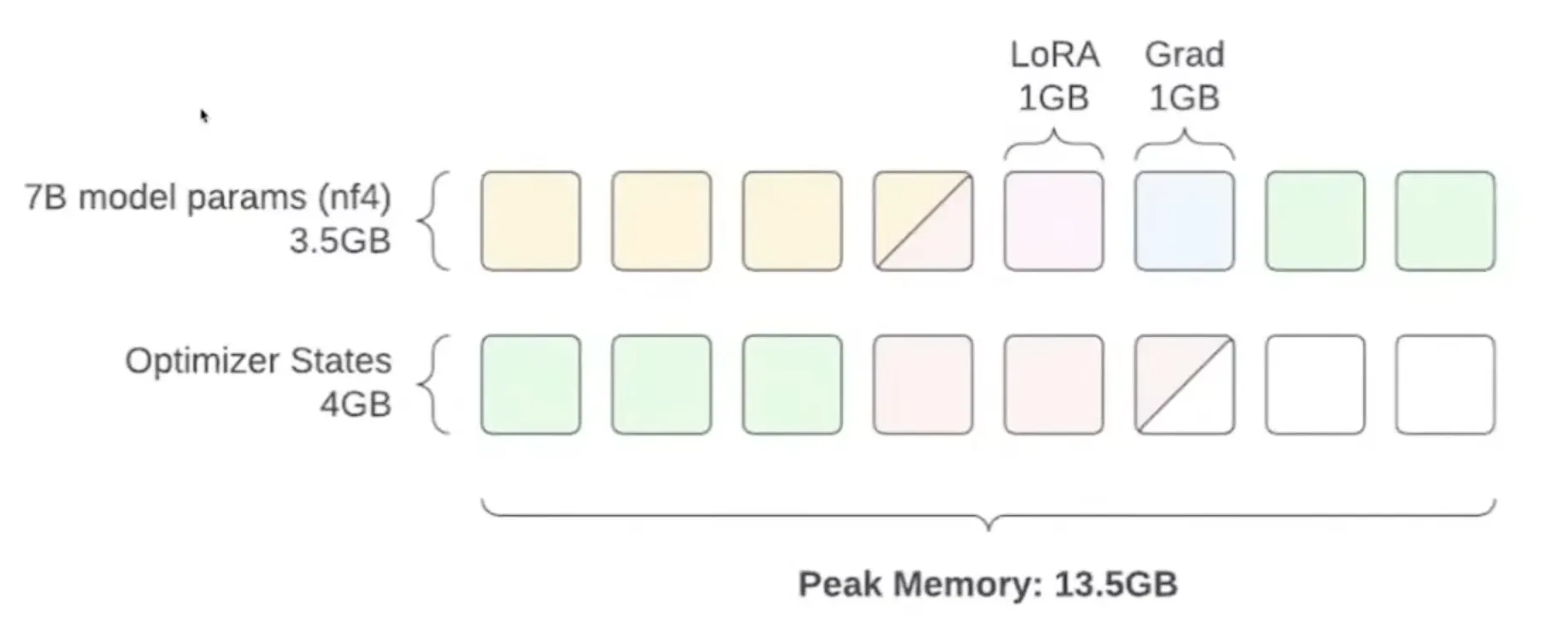
QLoRA

Can we use 4-bit quantization then? This is the idea proposed in the QLoRA paper. It uses a paged atom optimization technique to move optimizer state paged memory to the CPU when needed, reducing the impact of training peaks:

For this, a new unit nf4 (normal float 4) was introduced.

This saves even more VRAM:

Gradient Accumulation

The final issue lies in the choice of Batch Size. If we update using very few samples at a time, the variance during training will be high, with the extreme case being pure SGD. Usually, a middle ground is chosen, a sweet spot between large and smooth steps versus small and jerky steps, which is why batch sizes of 32, 64, or 128 are common.

But since we can only load one sample at a time, we use Gradient Accumulation.

The key idea is to achieve the training effect of using a larger batch size without increasing additional memory overhead.

The operations include:

1. Batching: Dividing a large batch of data into multiple small batches (determined based on available memory resources). For each small batch:

   • Perform a forward pass to calculate the loss.
   • Perform backpropagation to calculate gradients for the current small batch, but do not update model parameters immediately.

2. Gradient Accumulation: Accumulate the gradients calculated from each small batch into the previous gradients instead of using them to update parameters immediately.

3. Parameter Update: After processing all small batches and accumulating a sufficient number of gradients, use the accumulated gradients to update model parameters all at once.

Practical Fine-Tuning: Mistral 7B

QLoRA

16GB VRAM

Mixtral 8x7B (MoE)

Hardware requirement: >=65GB VRAM

Thanks for reading. I’ll update the practical fine-tuning section as soon as possible…