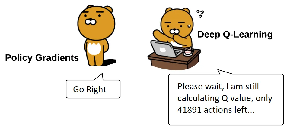
Exploring the evolution from value-based methods (DQN) to policy-based methods (Policy Gradient), and understanding the differences and connections between the two.
From DQN to Policy Gradient
:::note{title=“Review”} Q-Learning is an algorithm used to train the Q-function, which is an action-value function that determines the value of taking a specific action in a specific state. It maintains a Q-table to store memories of all state-action pair values. :::
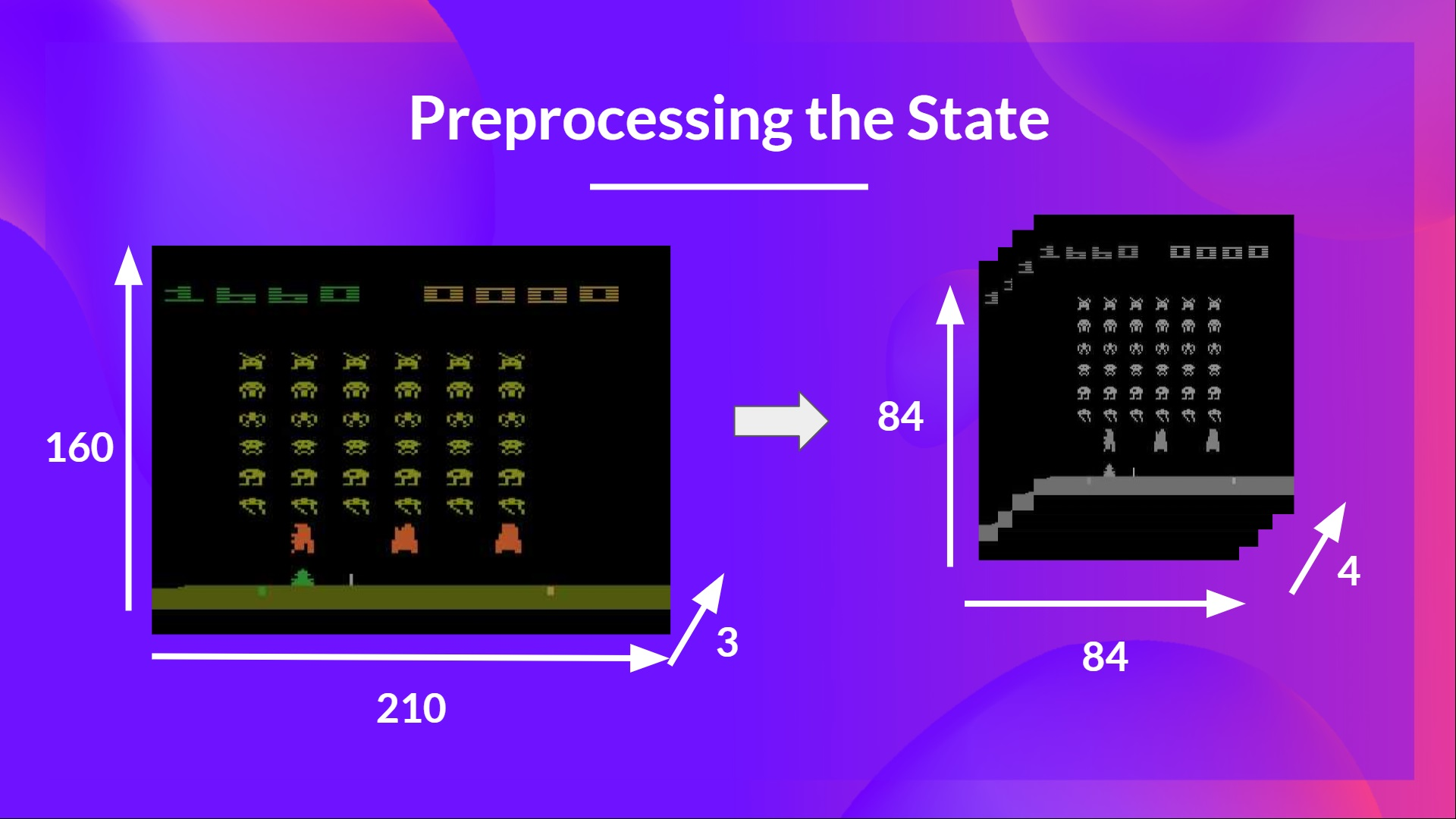
For Atari games like Space Invaders, we need to use game frames as states and inputs. A single frame is 210x160 pixels with 3 color channels (RGB). Thus, the observation space shape is (210, 160, 3). Each pixel value ranges from 0 to 255, leading to possible observations.
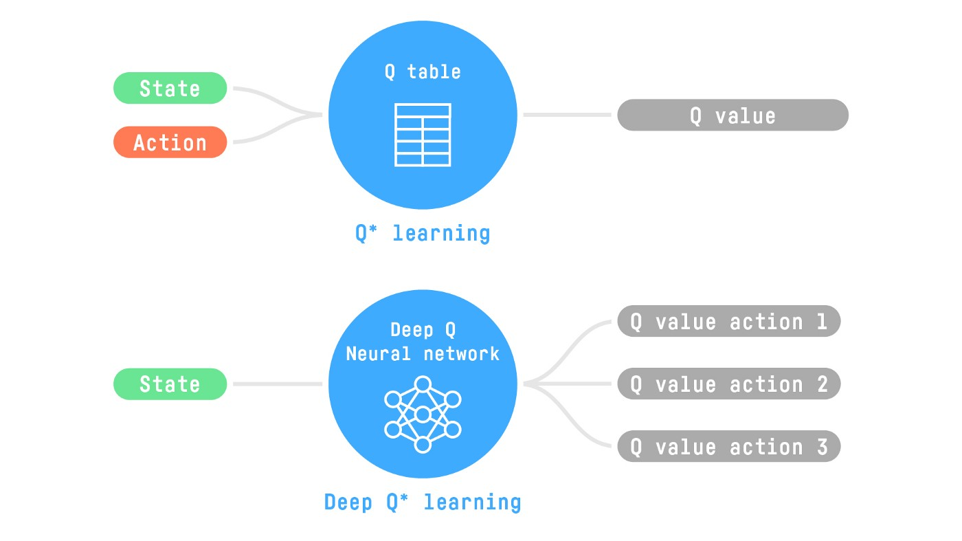
In such cases, generating and updating a Q-table is extremely inefficient. Therefore, we use Deep Q-Learning instead of tabular methods like Q-Learning, choosing a neural network as the Q-function approximator. This network approximates the Q-values for every possible action given a state.
DQN
Input Preprocessing and Temporal Limitations
We aim to reduce state complexity to decrease the computation time required for training.
Grayscaling
Color doesn’t provide essential information, so three color channels (RGB) can be reduced to one.
Screen Cropping
Regions that do not contain important information can be cropped out.
Capturing Temporal Information
Movement information (direction, speed) of a pixel cannot be determined from a single frame. To obtain temporal information, we stack four frames together.
CNN
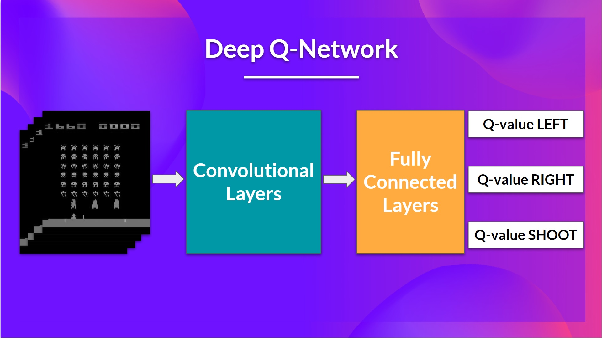
Stacked frames are processed through three convolutional layers to capture and utilize spatial relationships within the images. Additionally, because frames are stacked, we can obtain temporal information across frames.
MLP
Finally, fully connected layers serve as the output, providing a Q-value for each possible action in that state.
class QNetwork(nn.Module):
def __init__(self, env):
super().__init__()
self.network = nn.Sequential(
nn.Conv2d(4, 32, 8, stride=4),
nn.ReLU(),
nn.Conv2d(32, 64, 4, stride=2),
nn.ReLU(),
nn.Conv2d(64, 64, 3, stride=1),
nn.ReLU(),
self.network.add_module("Flatten", nn.Flatten()), # Flatten multidimensional input to 1D
nn.Linear(3136, 512), # Fully connected layer mapping 3136D input to 512D
nn.ReLU(),
nn.Linear(512, env.single_action_space.n), # Output layer corresponding to action space dimension
)
def forward(self, x):
return self.network(x / 255.0) # Normalize input to [0,1] range
Network Input: A 4-frame stack passed through the network as the state. Output: A vector of Q-values for each possible action in that state. Similar to Q-Learning, we then simply use an epsilon-greedy policy to choose which action to take.
During the training phase, we no longer directly update the Q-values of state-action pairs as in Q-Learning. Instead, we optimize the weights of the DQN by designing a loss function and using gradient descent.
Training Workflow
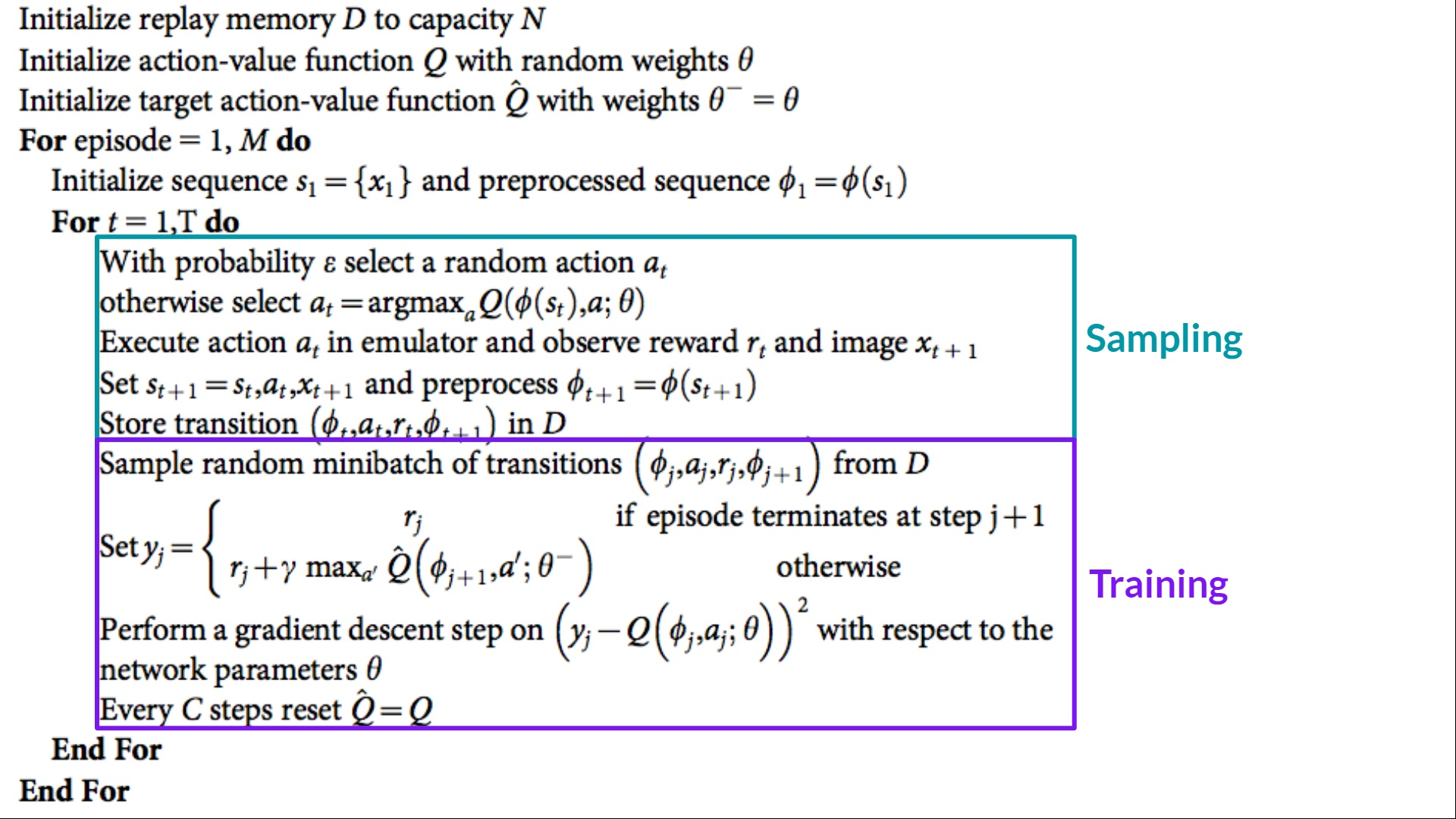
The Deep Q-Learning training algorithm has two phases:
- Sampling: Executing actions and storing the observed experience tuples in a replay buffer.
- Training: Randomly selecting a small batch of tuples and learning from that batch using a gradient descent update step.
Because Deep Q-Learning (off-policy) combines a non-linear Q-value function (neural network) with bootstrapping (updating targets using current estimates instead of actual complete returns, which is biased), its training process can be unstable. Sutton and Barto’s “deadly triad” refers to this exact situation.
Stabilizing Training
To help stabilize training, we implement three different solutions:
- Experience Replay for more efficient use of experience.
- Fixed Q-Targets to stabilize training.
- Double DQN to solve the problem of Q-value overestimation.
Experience Replay
Experience replay in Deep Q-Learning serves two functions:
- More efficient use of experience during training. In typical online reinforcement learning, an agent interacts with the environment to gain experience (state, action, reward, and next state), learns from it (updates the neural network), and then discards it, which is very inefficient. Experience replay helps by more efficiently utilizing training experience. We use a replay buffer to save experience samples so they can be reused during training.
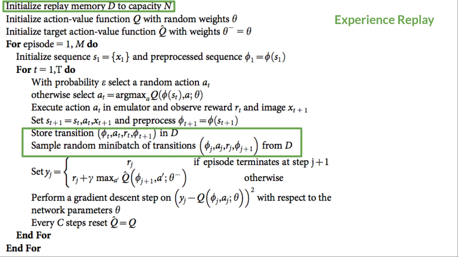
The agent can learn multiple times from the same experience.
- Avoid forgetting prior experience (catastrophic interference or catastrophic forgetting) and reduce the correlation between experiences. The Replay Buffer allows for storing experience tuples during interaction and then drawing small batches from them. This prevents the network from learning only the most recently executed actions. Randomly sampling experiences diversifies the data the agent is exposed to, preventing overfitting to short-term states and avoiding severe fluctuations or catastrophic divergence in action values.

Sampling experience and calculating loss:
rb = ReplayBuffer(
args.buffer_size, # Size of the replay buffer, determining how much experience to store.
envs.single_observation_space,
envs.single_action_space,
device,
optimize_memory_usage=True,
handle_timeout_termination=False,
)
if global_step > args.learning_starts:
if global_step % args.train_frequency == 0:
data = rb.sample(args.batch_size) # Randomly sample a batch
with torch.no_grad():
target_max, _ = target_network(data.next_observations).max(dim=1)
td_target = data.rewards.flatten() + args.gamma * target_max * (1 - data.dones.flatten())
old_val = q_network(data.observations).gather(1, data.actions).squeeze()
loss = F.mse_loss(td_target, old_val)Fixed Q-Targets
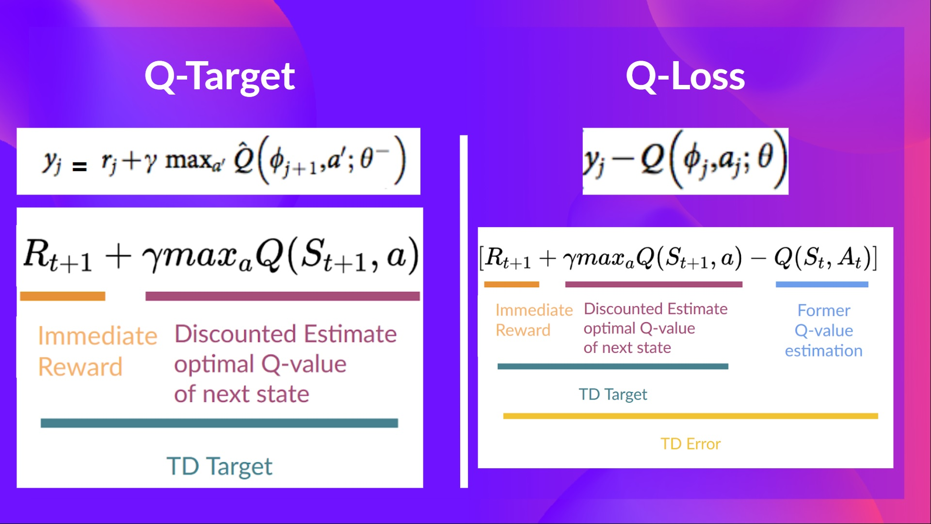
A key issue in Q-Learning is that parameters for the TD target (Q-Target) and the current Q-value (Q-estimate) are shared. This leads to both the Q-target and Q-estimate changing simultaneously, like chasing a moving target. A beautiful analogy is a cowboy (Q-estimate) trying to catch a moving cow (Q-target). Although the cowboy gets closer to the cow (error decreases), the target keeps moving, causing significant oscillations during training.

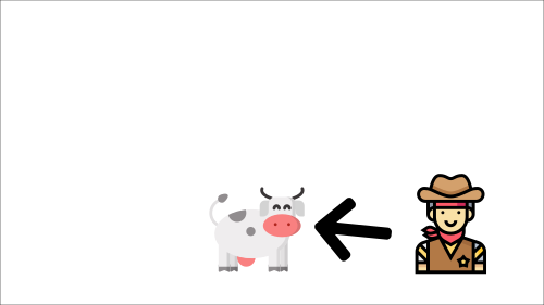
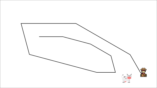
Love this representation 🥹
To solve this, we introduce Fixed Q-Targets. The core idea is to introduce an independent network that doesn’t update at every timestep but instead copies parameters from the main network every C steps. This means our target (Q-Target) remains fixed over multiple timesteps and the network is updated only against old estimates. This significantly reduces the oscillation between target and estimate.
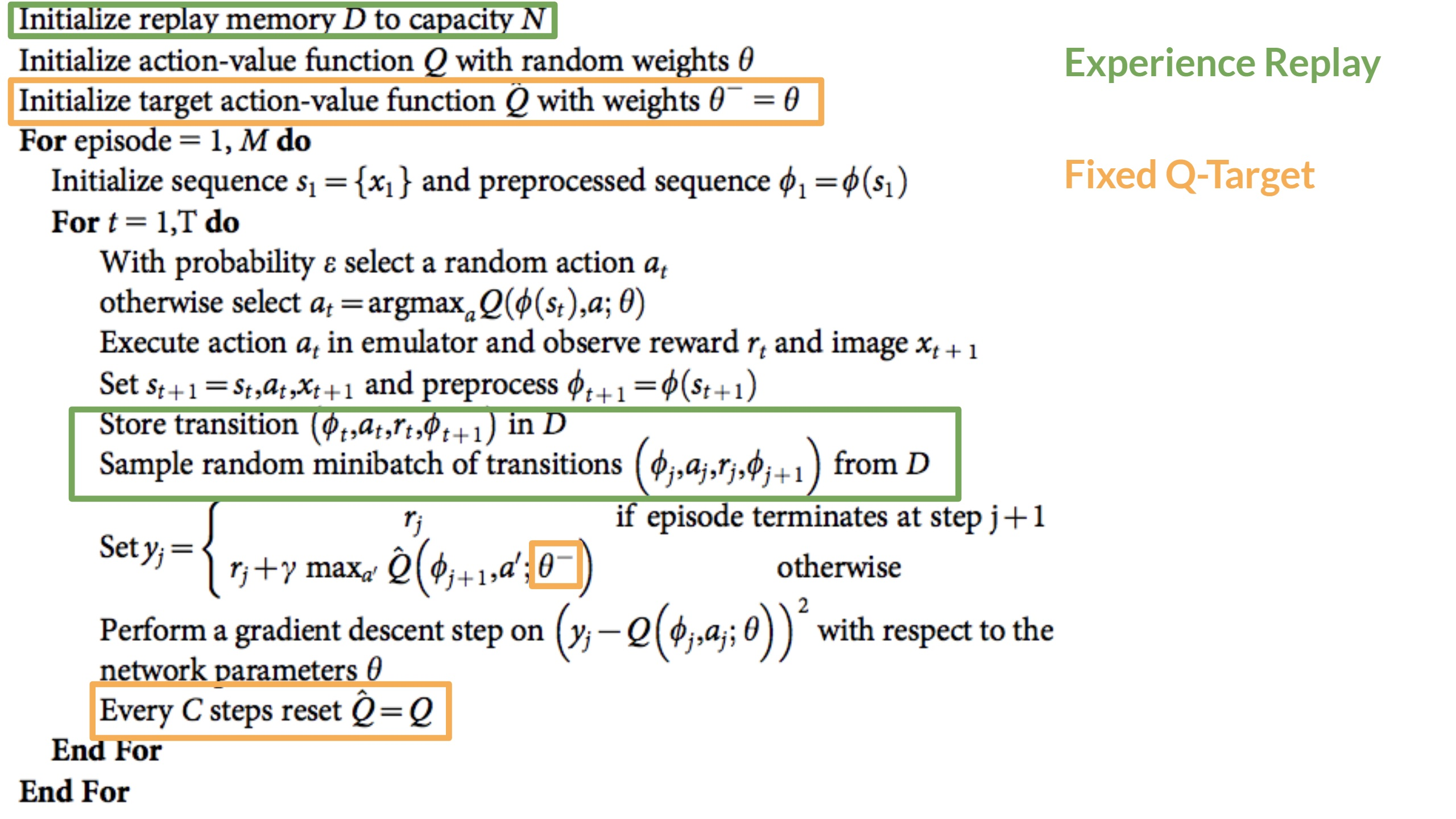
As shown in the pseudo-code above, the key is using two different networks: a main network (for choosing actions and updating) and a target network (for calculating Q-Targets), with main network weights copied to the target network every C steps. This stabilizes the training process, allowing the “cowboy to catch the cow more effectively,” reducing oscillations and speeding up convergence.
q_network = QNetwork(envs).to(device) # Current policy network, responsible for action selection and Q-value prediction
optimizer = optim.Adam(q_network.parameters(), lr=args.learning_rate)
target_network = QNetwork(envs).to(device) # Target network for calculating TD targets, providing stable learning goals.
target_network.load_state_dict(q_network.state_dict()) # Initialization: target network parameters match the current policy networkEvery args.target_network_frequency steps, the main network parameters are fully copied to the target network. This keeps the Q-Target fixed for multiple timesteps, significantly reducing the oscillation between target and estimate.
tau = 1.0
if global_step % args.target_network_frequency == 0:
for target_param, param in zip(target_network.parameters(), q_network.parameters()):
target_param.data.copy_(args.tau * param.data + (1.0 - args.tau) * target_param.data)Double DQN
Double DQN was proposed by Hado van Hasselt specifically to solve the problem of Q-value overestimation.
In Q-Learning TD-Target calculations, a common question is “How to determine if the best action for the next state is the one with the highest Q-value?” We know that Q-value accuracy depends on the actions we’ve tried and the neighboring states we’ve explored. Thus, early in training, information about the best action is insufficient. Choosing an action solely based on the highest Q-value can lead to misjudgment.
For instance, if a sub-optimal action is assigned a Q-value higher than the best action, the learning process becomes complicated and hard to converge. To address this, Double DQN introduces two networks to decouple action selection from Q-value target generation:
- Main Network (DQN Network): Used to select the best action for the next state (i.e., the action with the highest Q-value).
- Target Network: Used to calculate the target Q-value resulting from executing that action.
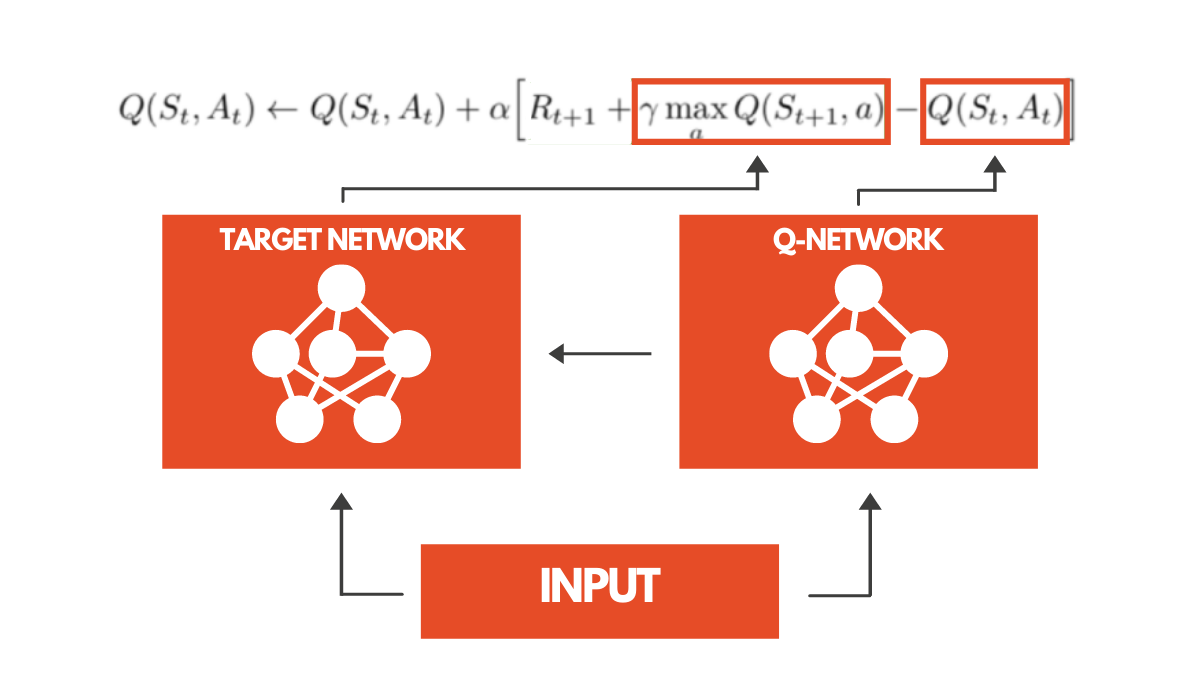
:::note{title=“Terminology”} Use the main network to select the best action, but use the target network to calculate the Q-value. This approach reduces Q-value overestimation and makes the training process more stable and efficient. :::
with torch.no_grad():
# Use main network to select the best action for the next state
next_q_values = q_network(data.next_observations)
next_actions = torch.argmax(next_q_values, dim=1, keepdim=True)
# Use target network to evaluate the Q-value of those actions
target_q_values = target_network(data.next_observations)
target_max = target_q_values.gather(1, next_actions).squeeze()
# Calculate TD-Target
td_target = data.rewards.flatten() + args.gamma * target_max * (1 - data.dones.flatten())
# Calculate current Q-value
old_val = q_network(data.observations).gather(1, data.actions).squeeze()
loss = F.mse_loss(td_target, old_val)Modern Deep Reinforcement Learning includes further improvements like Prioritized Experience Replay and Dueling Networks, which are not covered here.
Optuna
One of the most critical tasks in Deep Reinforcement Learning is finding a good set of training hyperparameters. Optuna is a library that helps you automate the search for the best hyperparameter combinations.
Policy Gradient
The previously mentioned Q-Learning and DQN are both value-based methods, which find optimal policies indirectly by estimating value functions. The existence of a policy () depends entirely on action-value estimates, as the policy is generated from the value function (e.g., a greedy policy choosing the action with the highest value in a given state).
In contrast, with policy-based methods, we aim to directly optimize the policy, bypassing the intermediate step of learning a value function. Next, we will dive into a subset called Policy Gradient.
In policy-based methods, optimization is mostly on-policy because for each update, we only use data (action trajectories) collected by the latest version of .
Parameterized Stochastic Policy
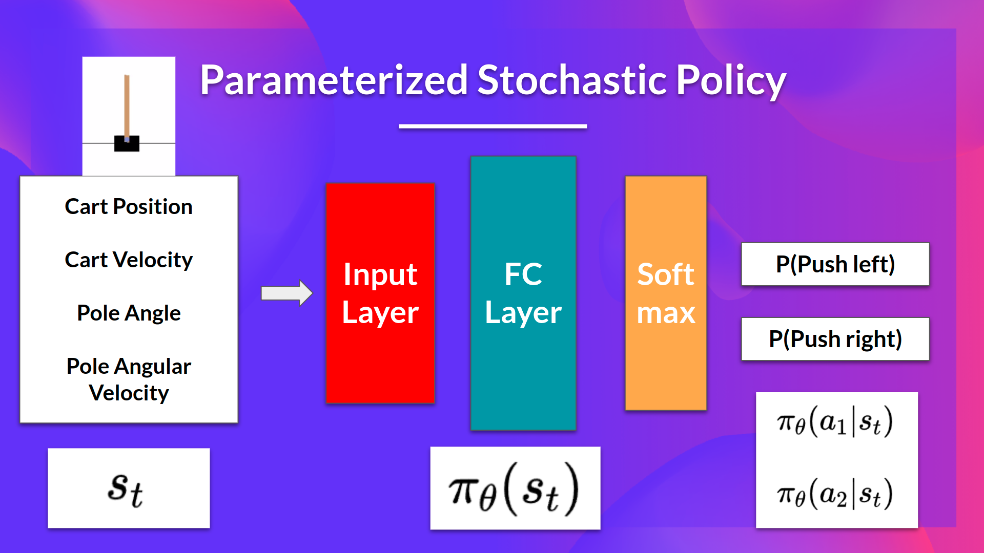
For example, having the neural network output an action probability distribution (stochastic policy) :
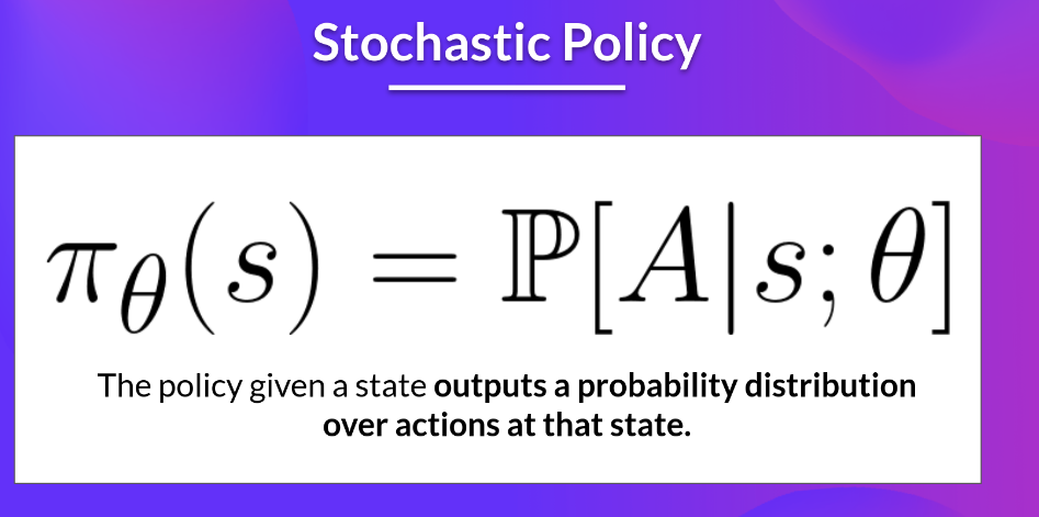
Objective function , optimization parameters . Maximize the performance of the parameterized policy through gradient ascent.
Advantages
Integration Convenience
- Policies can be estimated directly without storing additional data (action values); it can be understood as end-to-end.
Ability to Learn Stochastic Policies
Since the output is a probability distribution over actions, the agent can explore the state space without always following the same trajectories, eliminating the need to manually implement exploration/exploitation trade-offs. DQN learns a deterministic policy; we introduce randomness through tricks like ε-greedy, but this is not an inherent property of value-based methods. Simultaneously, it naturally handles state uncertainty, solving the problem of perceptual aliasing.
:::note{title=“Terminology”} Perceptual aliasing occurs when two states look (or are) identical but require different actions. :::
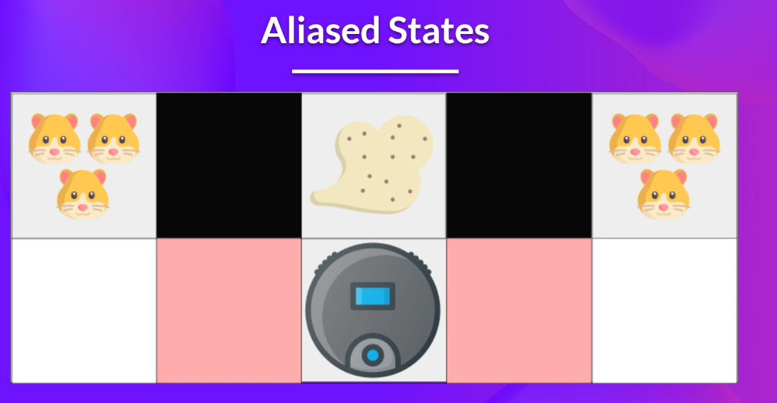
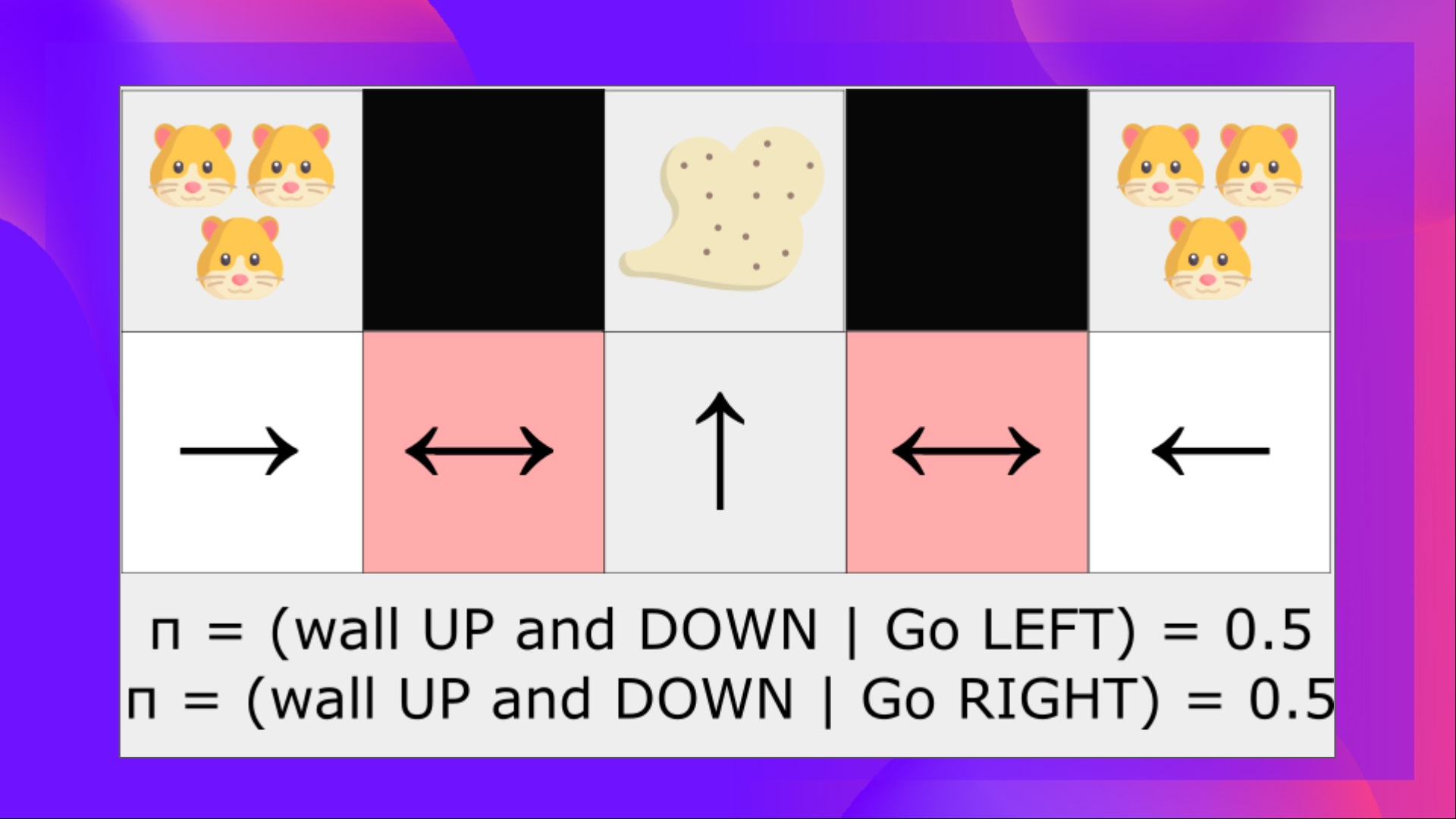
For example, in the scenario below, a vacuum cleaner agent must suck up dust while avoiding a hamster. The vacuum can only perceive the position of walls. In the diagram, these two red states are called “aliased states” because in these states, the agent perceives the same wall positions—walls both above and below. This leads to state ambiguity, making it impossible to distinguish which specific red state it is in.
Using a deterministic policy, the vacuum would always move right or left in a red state; if it chooses the wrong direction, it gets stuck in a loop. Even with an ε-greedy policy, the vacuum mainly follows the “best” policy but might repeatedly explore the wrong direction in an aliased state, leading to inefficiency.
Effective in High-Dimensional and Continuous Action Spaces
Policy gradient methods are particularly effective in high-dimensional or continuous action spaces.
An autonomous car might have infinitely many action choices in each state—turning the steering wheel by 15°, 17.2°, 19.4°, or other actions like honking. Deep Q-Learning would have to calculate a Q-value for every possible action, and finding the maximum Q-value in a continuous action space is itself an optimization problem. 
Better Convergence
In value-based methods, we update policies using to find the maximum Q-value. In this case, even a slight change in Q-values can lead to drastic changes in action selection. For instance, if the Q-value for turning left is 0.22 and then the Q-value for turning right becomes 0.23, the policy changes significantly, choosing right far more than left.
In policy gradient methods, action probabilities change smoothly over time, making the policy more stable.
Disadvantages
Local Optima
Often converges to local optima rather than the global optimum.
Low Training Efficiency
Training is slow and inefficient.
High Variance
Variance is large. We will explore the reasons and solutions for this later in Actor-Critic.
Detailed Analysis
Policy gradient adjusts parameters (the policy) with each interaction between the agent and the environment, allowing the action probability distribution to sample more “good” actions that maximize returns.
Objective Function
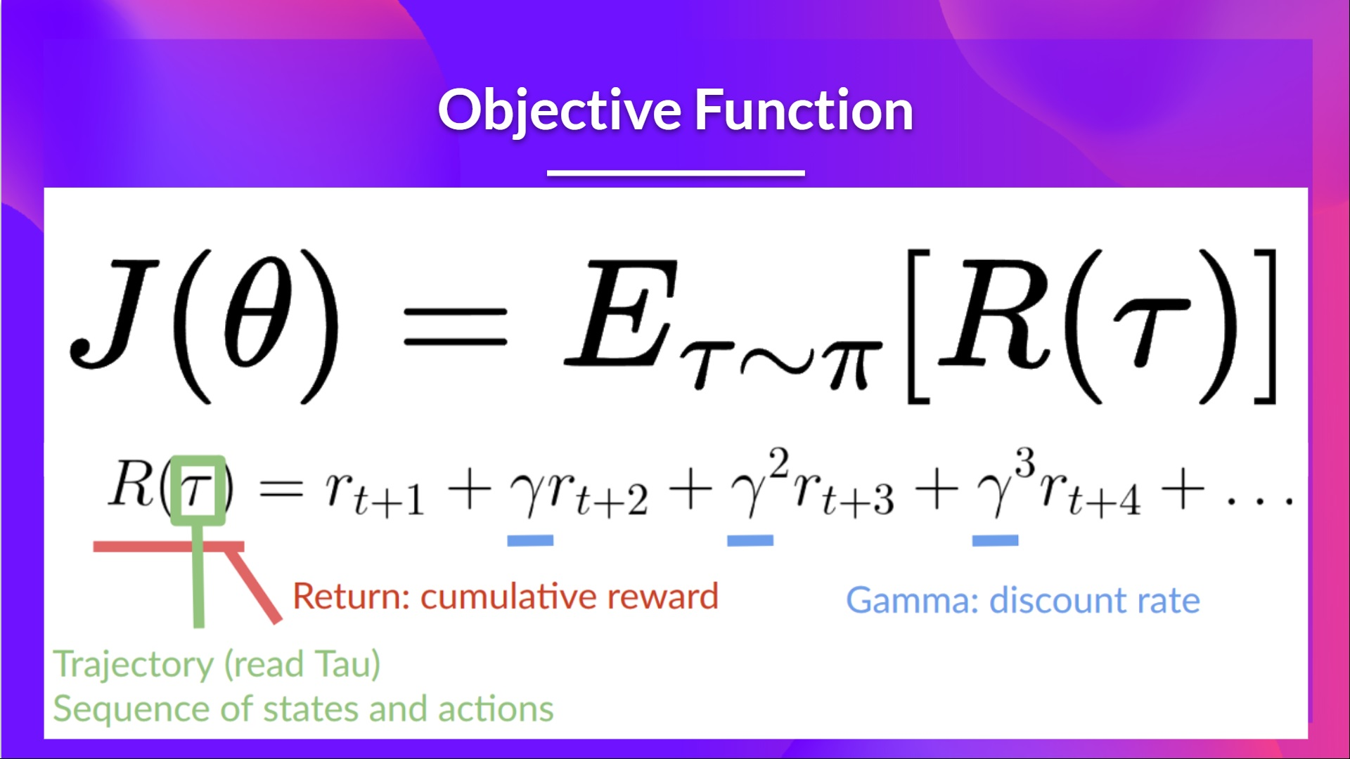
Our goal is to find parameters that maximize the expected return:
Since this is a concave function (we want to maximize the value), we use gradient ascent: .
However, the true gradient of the objective function is uncomputable because it requires calculating probabilities for every possible trajectory, which is computationally expensive. Therefore, we aim to calculate a gradient estimate through sample-based estimation (collecting some trajectories).
Additionally, the state transition probabilities (or state distribution) of the environment are often unknown. Even if known, they are complex and non-linear, making it impossible to directly calculate derivatives. In other words, we cannot directly differentiate the state transition dynamics (controlled by a Markov Decision Process) to optimize the policy.
Policy Gradient Theorem
A full derivation can be found on Andrej Karpathy’s blog, and I’ve also summarized my learning here: Introduction to Policy Gradient 6. PG Derivation
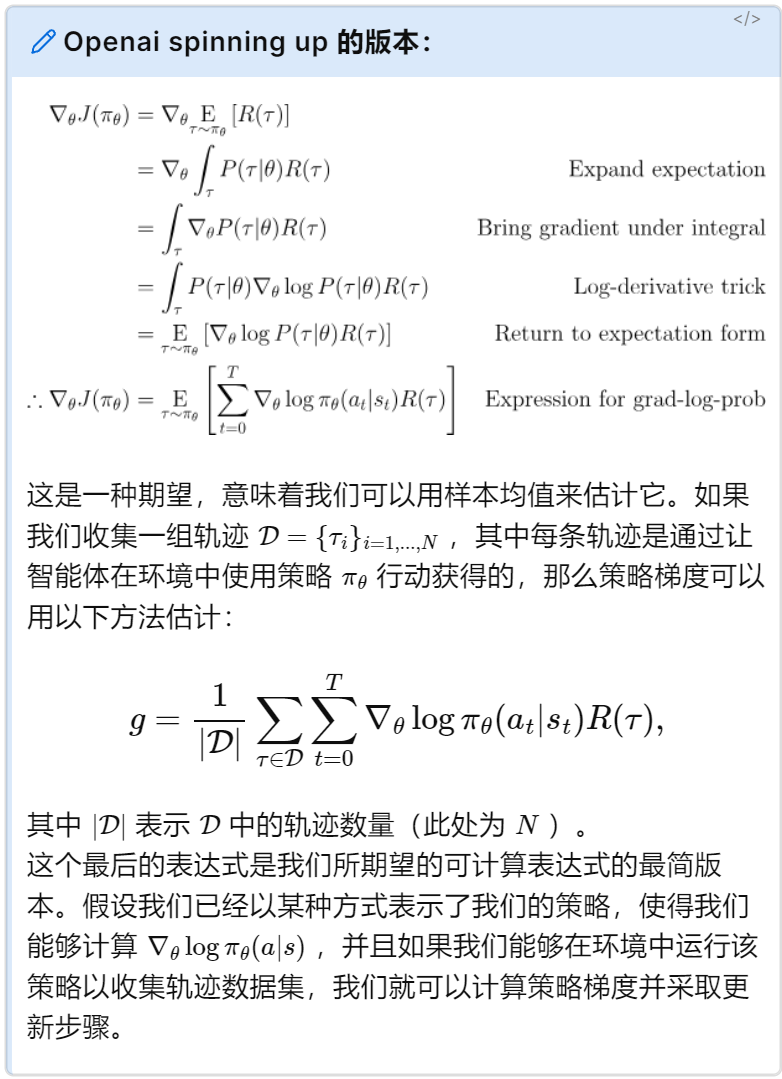
REINFORCE Algorithm (Monte Carlo Policy Gradient)
Utilizes the estimated return of an entire episode to update policy parameters . Collect an episode using policy , and use that episode to estimate the gradient . Optimization: .
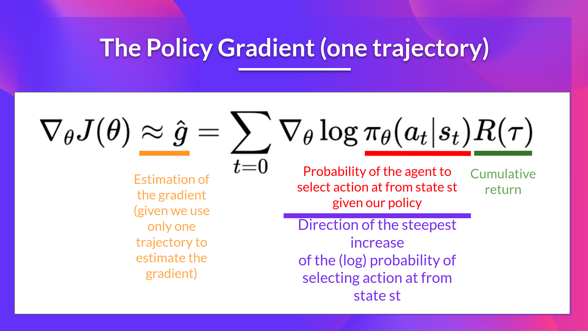
: This part represents the gradient of the log probability of an action given a state and action . We aren’t calculating a specific action value (Q-value).
: Here is the cumulative return over the entire trajectory , used to measure the total reward after executing policy . A high return increases the probability of the (state, action) combination, while a low return decreases it.
We can also collect multiple episodes (trajectories) to estimate the gradient: 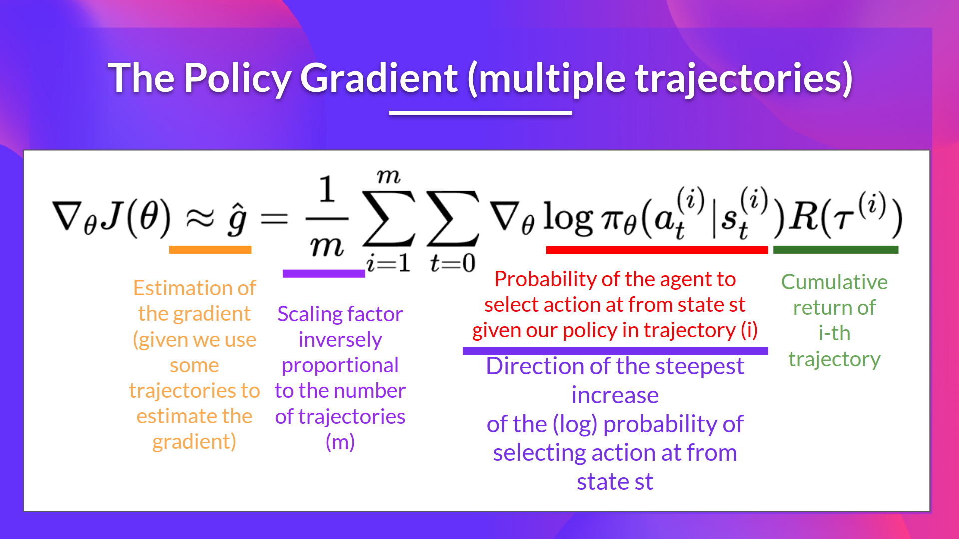
References