The Intuition and Mathematics of Diffusion

https://www.youtube.com/watch?v=HoKDTa5jHvg

This article primarily follows the teaching logic of this video, organized and elaborated with explanations. If there are any errors, feel free to correct them in the comments!

Intuition Part

Theoretical Support

Deep Unsupervised Learning using Nonequilibrium Thermodynamics

This paper laid the theoretical foundation for diffusion models. The authors proposed a generative model based on non-equilibrium thermodynamics that achieves data generation by step-wise adding and removing noise. This provided crucial theoretical support for subsequent research in diffusion models.

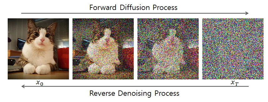
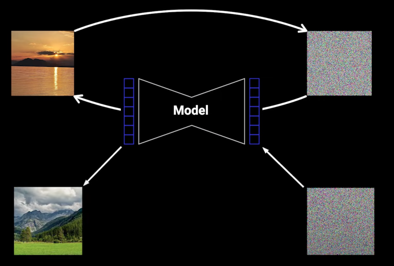
We apply a large amount of noise to images and then use a neural network to denoise them. If this neural network learns well, it can start from completely random noise and eventually obtain an image from our training data.

Forward Diffusion Process:

Iteratively applying noise to an image. Given enough steps, the image turns completely into noise. Normal distribution is used as the noise source:

Reverse Diffusion Process

From pure noise to an image, involving a neural network that learns to denoise step by step.

Why denoising gradually? The authors mentioned in the paper that the result of “one-step direct denoising” is poor.

So what does this network look like? And what is it supposed to predict?

Algorithm Improvement

Denoising Diffusion Probabilistic Models

This paper proposed Denoising Diffusion Probabilistic Models (DDPM), significantly improving the generation quality and efficiency of diffusion models. By introducing a simple denoising network and optimized training strategies, DDPM became an important milestone in the field.

The authors discussed three possible targets for the neural network to predict:

1. Predict the mean of the noise at each timestep (predict the mean of the noise at each timestep)

   • Predicting the mean of the conditional distribution $p(x_{t-1}|x_t)$
   • Variance is fixed and non-learnable

2. Predict $x_0$ directly (predict $x_0$ directly)

   • Directly predicting the original, uncorrupted image
   • Experiments showed this method performs poorly

3. Predict the added noise (predict the added noise)

   • Predicting the noise $ε$ added during the forward process
   • Mathematically equivalent to the first method (predicting the noise mean), just a different parameterization; they can be transformed into each other through simple operations

The paper ultimately chose predicting noise (the third way) as the primary method because it is more stable to train and yields better results.

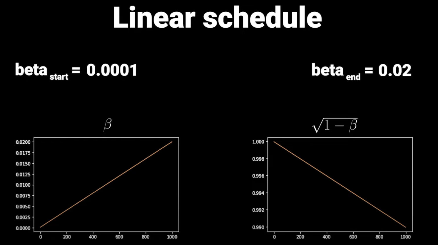
The amount of noise added at each step is not constant; it’s controlled by a Linear Schedule to prevent training instability.

It looks something like this:

As seen, the last few timesteps are close to complete noise with very little information. Furthermore, looking at the whole process, information is destroyed too quickly. OpenAI solved these two problems using a Cosine Schedule:

Model Architecture

U-Net

Published alongside this paper was a model architecture called U-Net:

This model features a Bottleneck in the middle (layers with fewer parameters). It uses Downsample-Blocks and Resnet-Blocks to project the input image to a lower resolution, and Upsample-Blocks to project it back to its original size.

At certain resolutions, the authors added Attention-Blocks and used Skip-Connections between layers in the same resolution space. The model is designed to target each timestep, implemented through sinusoidal positional encoding embeddings from Transformers, which are projected into each Residual-Block. The model can also combine schedules to remove different amounts of noise at different timesteps to improve generation.

Bottleneck and Autoencoder

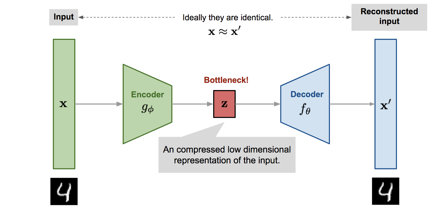
The concept of a Bottleneck was originally proposed and widely used in the unsupervised learning method “Autoencoder.” As the lowest-dimensional hidden layer in an Autoencoder architecture, it sits between the encoder and decoder, forming the narrowest part of the network. This forces the network to learn a compressed representation of data, minimizing reconstruction error and acting as regularization: $\mathcal{L}_{\text{reconstruction}} = \|X - \text{Decoder}(\text{Encoder}(X))\|^2$

Architectural Improvements

OpenAI significantly improved overall results in their second paper Diffusion Models Beat GANs on Image Synthesis through architectural improvements:

1. Increased network depth (more layers), decreased width (channels per layer)
2. Increased the number of Attention-Blocks
3. Expanded the number of heads in each Attention Block
4. Introduced BigGAN-style Residual Blocks for upsampling and downsampling
5. Introduced Adaptive Group Normalization (AdaGN), dynamically adjusting normalization parameters based on conditional information (like timesteps)
6. Used Separate Classifier Guidance to help the model generate specific classes of images

Mathematics Part

Symbol Table

• $X_t$ represents the image at timestep $t$, where $X_0$ is the original image. Note that smaller $t$ means less noise:

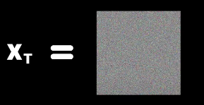
• The final noisy image is an isotropic (same in all directions) total noise, denoted as $X_T$. In initial research $T=1000$, but later work reduced this significantly:

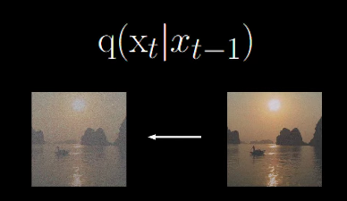
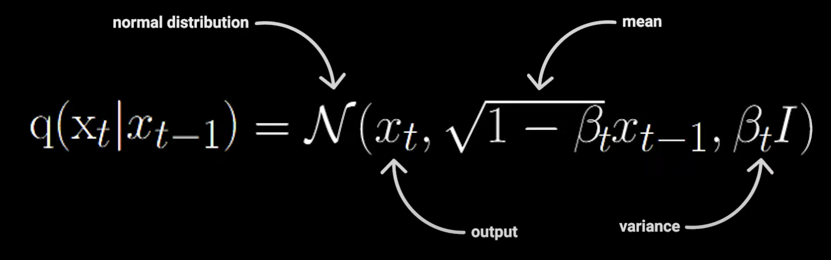
• Forward Process: $q(x_t|x_{t-1})$, taking $x_{t-1}$ and outputting a noisier image $X_t$:

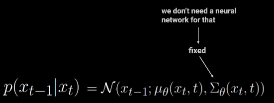
• Backward Process: $p(x_{t-1}|x_t)$, taking $x_t$ and using a neural network to output a denoised image $x_{t-1}$:

Forward Process

Where:

• $\sqrt{1 - \beta_t} x_{t-1}$ is the mean of the distribution; $\beta_t$ is the noise schedule parameter, ranging from 0 to 1. Combined with $\sqrt{1 - \beta_t}$, it scales the noise. It decreases as the timestep increases, representing the retained part of the original signal.

• $\beta_t I$ is the covariance matrix of the distribution. $I$ is the identity matrix, indicating the covariance matrix is diagonal with independent dimensions. As the timestep increases, the amount of added noise grows.

Now we just need to iteratively execute this step to get the result after 1000 steps, but it can actually be done in one go.

Reparameterization Trick

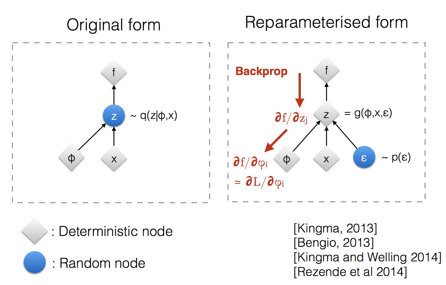
The reparameterization trick is very important in diffusion models and other generative models (like Variational Autoencoders, VAE). Its core idea is transforming the sampling process of a random variable into a deterministic function plus a standardized random variable. This transformation allows the model to be optimized through gradient descent because it eliminates the impact of randomness in the sampling process on gradient calculation.

Here’s a simple example to explain its significance:

There are two ways to implement rolling a die.

• The first has randomness inside the function:

# 1. Direct die roll (random sampling)
def roll_dice():
    return random.randint(1, 6)
 
result = roll_dice()

• The second separates randomness outside, keeping the function deterministic:

# 2. Separating randomness
random_number = random.random()  # Generate random number between 0 and 1
 
def transformed_dice(random_number):
    # Map 0-1 random number to 1-6
    return math.floor(random_number * 6) + 1
 
result = transformed_dice(random_number)

In probability theory, we learn: if $X$ is a random variable and $X \sim \mathcal{N}(0,1)$, then $aX + b \sim \mathcal{N}(b, a^2)$.

Therefore, for a normal distribution $\mathcal{N}(\mu, \sigma^2)$, samples can be generated as:

where $\epsilon \sim \mathcal{N}(0, 1)$ is the standard normal distribution.

Similarly, for normal distributions:

• Without Reparameterization:

# Sample directly from the target normal distribution
x = np.random.normal(mu, sigma)

• With Reparameterization:

# Sample from standard normal distribution first
epsilon = np.random.normal(0, 1)
# Then get the target distribution via deterministic transformation
x = mu + sigma * epsilon

When it comes to gradient calculation in model training:

Without Reparameterization:

def sample_direct(mu, sigma):
    return np.random.normal(mu, sigma)
 
# In this case, it's hard to calculate gradients w.r.t. mu and sigma
# because random sampling blocks gradient propagation

With Reparameterization:

def sample_reparameterized(mu, sigma):
    epsilon = np.random.normal(0, 1)  # Gradient doesn't flow through here
    return mu + sigma * epsilon        # Easy to calculate gradients for mu and sigma

Taking VAE as an example:

class VAE(nn.Module):
    def __init__(self):
        super(VAE, self).__init__()
        self.encoder = Encoder()  # Outputs mu and sigma
        self.decoder = Decoder()
 
    def reparameterize(self, mu, sigma):
        # Reparameterization trick
        epsilon = torch.randn_like(mu)  # Sample from standard normal distribution
        z = mu + sigma * epsilon        # Deterministic transformation
        return z
 
    def forward(self, x):
        # Encoder outputs mu and sigma
        mu, sigma = self.encoder(x)
        
        # Use reparameterization to sample
        z = self.reparameterize(mu, sigma)
        
        # Decoder reconstructs input
        reconstruction = self.decoder(z)
        return reconstruction

Reparameterization from a Foodie’s Perspective

Imagine making milk tea:

Without Reparameterization:

• You make a cup of milk tea with a specific sweetness directly.
• If it’s not good, you don’t know if you added too much sugar or too little water.

With Reparameterization:

1. Prepare a standard concentration of sugar water first ($\epsilon$).
2. Then adjust the amount of sugar water ($\mu$) and dilution degree ($\sigma$) to reach the target sweetness.
3. If it’s not good, you clearly know whether the sugar water amount or dilution needs adjusting (parameters can be optimized).

In summary, via reparameterization:

• Gradients can propagate through deterministic transformations.
• Parameters can be optimized via gradient descent.
• Randomness is isolated and doesn’t affect gradient calculation.

Forward Mathematical Derivation

Transition from $x_{t-1}$ to $x_t$:

• Given $x_{t-1}$, we want to generate $x_t$.
• Applying the reparameterization trick to $q(x_t \mid x_{t-1}) = \mathcal{N}(x_t; \sqrt{1 - \beta_t} x_{t-1}, \beta_t I)$,

We can express $x_t$ as a deterministic transformation of $x_{t-1}$ plus a noise term:

• Here, $\sqrt{1 - \beta_t} x_{t-1}$ is the mean part, and $\sqrt{\beta_t} \epsilon$ is the noise part. Since $\epsilon$ is a sample from a standard normal distribution and independent of model parameters, gradients only need to consider the parameters corresponding to $\sqrt{1 - \beta_t}$ and $\sqrt{\beta_t}$ during backpropagation. This allows the model to be effectively optimized via gradient descent.

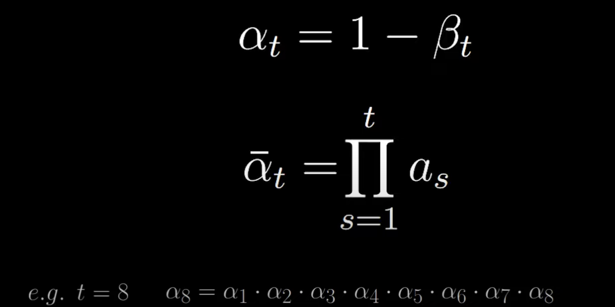
We use $\alpha_t$ to simplify notation and record the cumulative product:

Resulting in:

Calculating a two-step transition: from $x_{t-2}$ to $x_t$:

Since $\epsilon_{t-1}$ and $\epsilon_t$ are independent standard normal distributions, we can merge the noise parts into a single new noise term $\epsilon \sim \mathcal{N}(0, I)$:

Similarly:

The full derivation flow is as follows:

Reverse Mathematical Derivation

Since variance is fixed and doesn’t need learning (see section 1.3), we only need the neural network to predict the mean:

Our ultimate goal is to predict the noise between two timesteps. Let’s start analyzing from the loss function:

However, in this negative log-likelihood, the probability of $x_0$ depends on all other preceding timesteps. We can learn a model that approximates these conditional probabilities as a solution. Here we need the Variational Lower Bound to get a more computable formula.

Variational Lower Bound

Suppose we have an uncomputable function $f(x)$—in our case, the negative log-likelihood. We can find a computable function $g(x)$ that always satisfies $g(x) \leq f(x)$: Optimizing $g(x)$ will also increase $f(x)$:

We ensure this by subtracting the KL Divergence, a metric that measures the similarity between two distributions, which is always non-negative:

Subtracting an always non-negative term ensures the result is always less than the original function. We use ”+” here because we want to minimize the loss, so adding it ensures it’s always greater than or equal to the original negative log-likelihood:

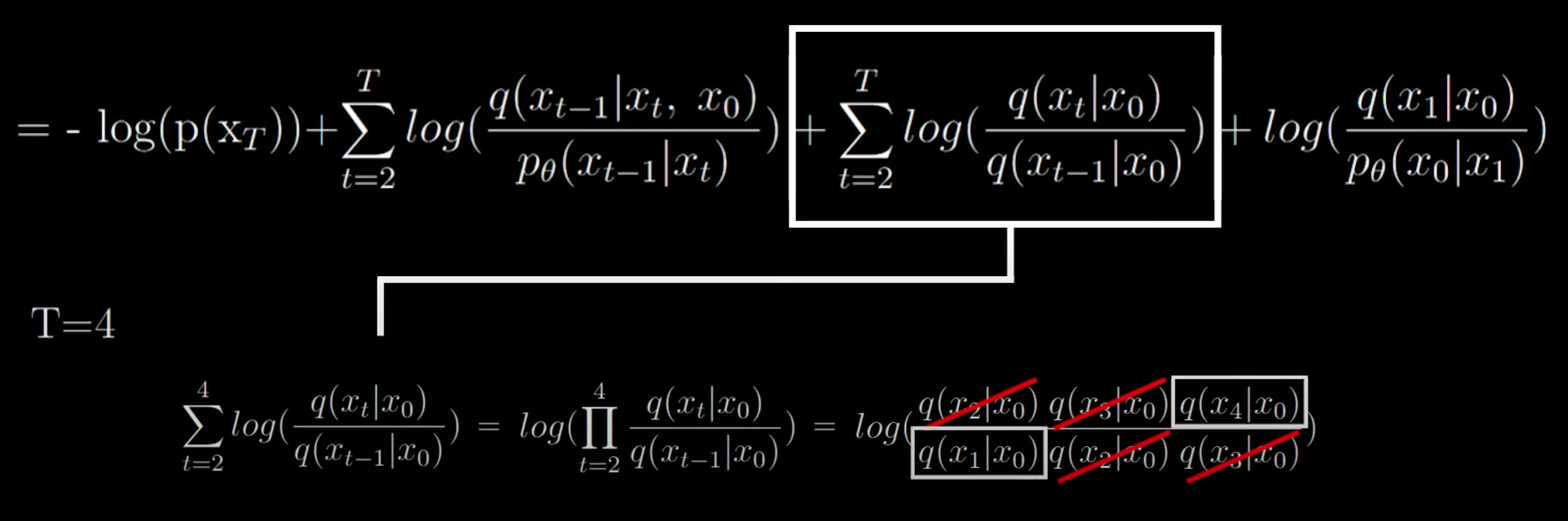
In this form, since the negative log-likelihood is still present, the lower bound remains uncomputable. We need a better expression. First, rewrite the KL divergence as a log ratio of two terms:

Next, apply Bayes’ rule to the denominator:

[!NOTE] Bayes’ Rule: $p(A \mid B) = \frac{p(B \mid A) p(A)}{p(B)}$

The numerator part $p_\theta(x_0 \mid x_{1:T}) p_\theta(x_{1:T})$ is actually the joint probability $p_\theta(x_0, x_{1:T})$, because:

Usually, $p_\theta(x_{0:T})$ represents the joint probability of $x_0$ and all intermediate steps $x_{1:T}$, i.e.:

[!NOTE] $p_\theta(x_{0:T})$ represents the joint probability distribution of all states $x_0, x_1, \ldots, x_T$ from timestep 0 to $T$.

$$p_\theta(x_{0:T}) = p(x_T) \prod_{t=1}^T p_\theta(x_{t-1} \mid x_t)$$

Substituting gives:

Following the process below leads to the final form:

Now the two problematic terms cancel out:

This gives us a lower bound that can be minimized, and all parts are known:

• The numerator is the joint probability of the forward process: $q(x_{1:T} \mid x_0)=\prod_{t=1}^T q(x_t \mid x_{t-1})$;
• The denominator is the joint probability of the reverse process: $p_\theta (x_{0:T})=p(x_T) \prod_{t=1}^T p_\theta(x_{t-1} \mid x_t)$

To make it analytically solvable, a few more reorganization steps are needed:

Rewrite the numerator of the sum term using Bayes’ rule: $q(x_t \mid x_{t-1})=\frac{q(x_{t-1}\mid x_t)q(x_t)}{q(x_{t-1})}$

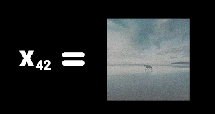
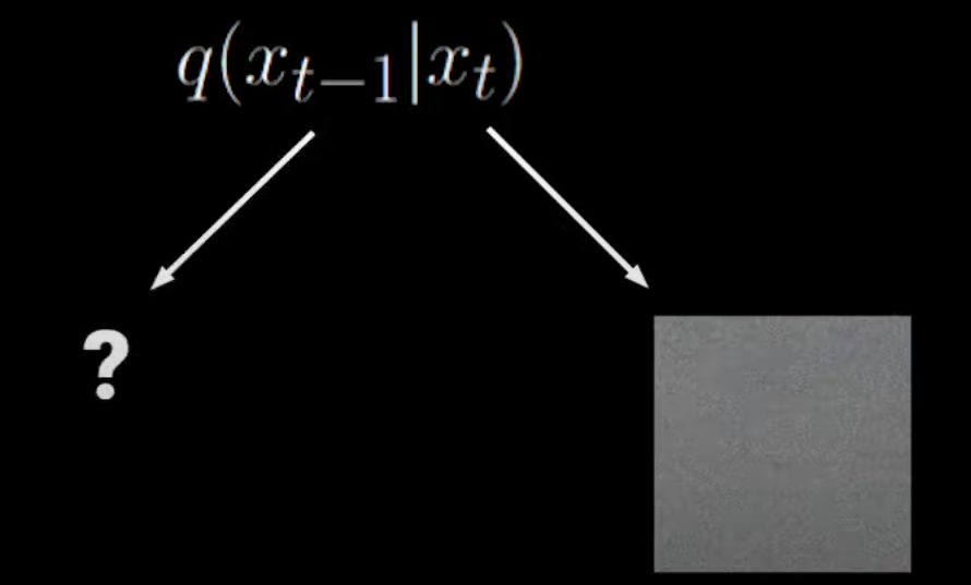
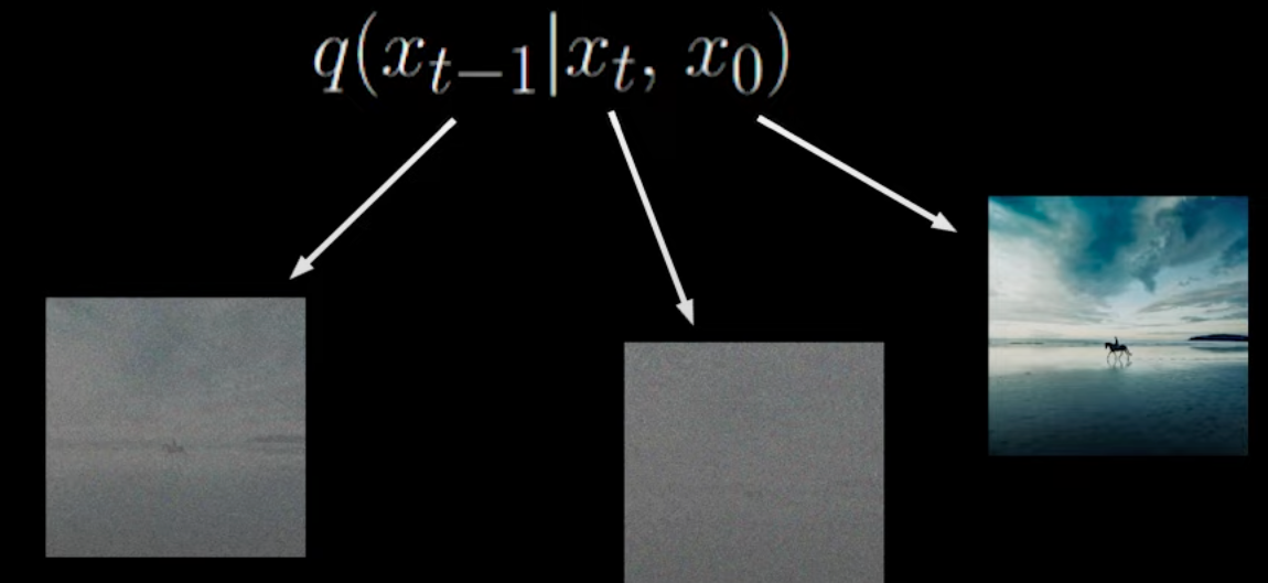
But this goes back to before, where these terms require estimating all samples, leading to high variance. As shown in the image below, given $x_t$, it’s hard to determine what the previous state looked like:

The improvement strategy is to condition directly on the original data $x_0$:

By providing the noiseless image simultaneously, there are fewer candidate $x_{t-1}$ states, reducing variance:

Substituting back:

Expanding the second sum, most terms cancel out:

Applying log rules to the last two terms simplifies them:

Moving the first simplified term to the front and merging into a logarithm yields the final analytical form:

The first term can be ignored because $q$ has no learnable parameters—it’s just the noise-adding forward process that converges to a normal distribution. $p(x_T)$ is just noise sampled from a Gaussian distribution, so the KL divergence will be very small.

The derivation of the remaining two terms is as follows (process omitted, see Lilian’s blog for details):

Since $\beta$ is fixed, we focus on the form of $\mu$:

The closed form generated by the forward process $x_t = \sqrt{\bar{\alpha}_t} x_0 + \sqrt{1 - \bar{\alpha}_t} \epsilon$ can be rewritten in terms of $x_0$:

Substituting this $x_0$ expression into the predicted mean formula $\tilde{\mu}_t$:

Now $\mu$ no longer depends on $x_0$. Continuing to simplify, first expand the second term:

Merging the $x_t$ terms:

Further merging and simplifying the coefficient for $x_t$ leads to:

This means we essentially just subtract the randomly scaled noise generated by $x_t$, which is what the neural network needs to predict.

Substituting into the loss function $L_t$, defined as Mean Squared Error:

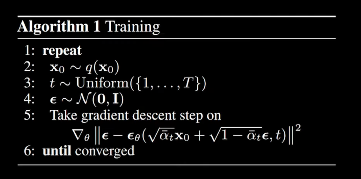
The final form is the mean squared error between the actual noise at timestep $t$ and the noise predicted by the neural network. Researchers found that ignoring the preceding scaling term results in better sampling quality and is easier to implement.

Going back to the original formula:

The authors decided not to add extra random noise in the final sampling step to stabilize the generation process:

The final form is:

• $\mathbb{E}_{t, \mathbf{x}_0,\boldsymbol{\epsilon}}$ denotes the expectation over timestep $t$, original data $\mathbf{x}_0$, and noise $\boldsymbol{\epsilon}$.
• $\boldsymbol{\epsilon}$ is the actual random noise added.
• $\boldsymbol{\epsilon}_\theta$ is the noise predicted by the neural network.
• $\sqrt{\bar{\alpha}_t} \mathbf{x}_0 + \sqrt{1 - \bar{\alpha}_t} \boldsymbol{\epsilon}$ is the closed-form solution of the forward process, representing noisy data at timestep $t$, thus simplifying to:
  • $\mathbf{x}_t$ directly represents noisy data at timestep $t$.
  • The entire loss function essentially measures the mean squared error between predicted and actual noise.

Timestep $t$ is usually sampled from a uniform distribution ($t \sim Uniform(1,T)$). This choice ensures that during training, every timestep has an equal probability of being selected, allowing the model to effectively learn the denoising process across all timesteps.

Training

First, we sample images from the dataset, then sample $t$ and noise from a normal distribution, and finally optimize the objective via gradient descent.

Sampling

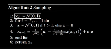
First, sample $x_t$ from a normal distribution, then sample $x_{t-1}$ via reparameterization using the formula shown earlier.

Note that no noise is added when $t=1$. According to the formula:

At $t=1$, the formula is used to recover $x_0$ from $x_1$, the final step of the denoising process. At this point, we want to reconstruct the original image as accurately as possible. Not adding noise at the last step (i.e., no $\sqrt{\beta_t} \epsilon$ term) avoids introducing unnecessary randomness into the final generated image, maintaining clarity and detail.

Code Implementation

Recommend Sunrise’s simplified MLP implementation on Zhihu. Later, when I have time, I’ll consider doing a manual implementation of Stable Diffusion. Digging a hole for myself…

References

• Diffusion Models | Paper Explanation | Math Explained
• Lilian Weng: From Autoencoder to Beta-VAE
• Lilian Weng: What are Diffusion Models?