Visual Language Models, with PaliGemma as a Case Study

Huge thanks to Umar Jamil for the great explanations in this video tutorial.

Vision-language models can roughly be divided into four categories $^{[1]}$ :

Turn images into embeddings that can be jointly trained with text tokens, such as VisualBERT, SimVLM, CM3, etc.
Learn strong image embeddings and use them as a prefix for a frozen pretrained autoregressive model, such as ClipCap.
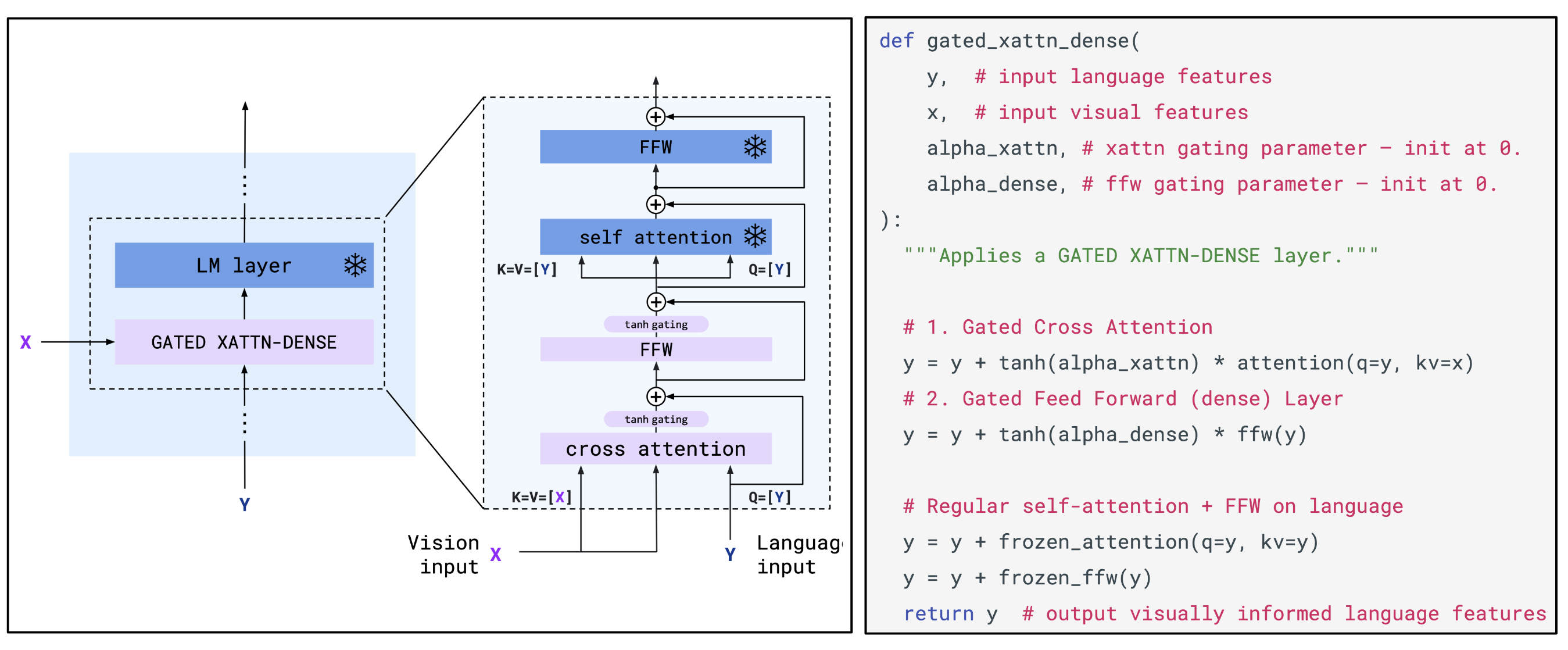
Fuse visual information into the language model’s layers via dedicated cross-attention, such as VisualGPT and Flamingo (see figure below)
Combine a vision model and a language model without any training, such as MAGiC (guided decoding)

A VLM is made up of a Vision Encoder, a Linear Projection Layer, and an LLM Decoder. The key problem is how to merge image-token embeddings with text-token embeddings, so the model can produce the right output conditioned on the inputs.

Screenshot 2025-05-10 at 02.31.36

Vision Encoder

ViT

Vision Transformer (ViT) combines computer vision with the Transformer architecture, using a pure Encoder stack for image classification. The core idea is to split an image into fixed-size patches, then convert those patches into vision embeddings as the Transformer’s input sequence.

Each patch gets a learnable positional embedding to preserve spatial information. Since ViT uses bidirectional attention rather than an autoregressive setup (so no attention mask is needed), each patch embedding can encode not only its own content but also contextual information from other patches via self-attention—yielding contextualized representations. This design helps the model relate global semantics to local features.

Screenshot 2025-05-22 at 22.18.41

The special 0* token is the classification marker ([class] token) used for classification tasks.

This turns the image into a sequence of embeddings, one per patch. These can be concatenated with text-token embeddings and fed into an LLM. The key technique involved here is contrastive learning.

CLIP

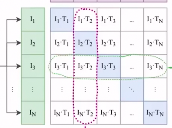
In simple terms, you train on a dataset of images and their corresponding text descriptions. Given a batch of image–text pairs, the goal of contrastive learning (as in CLIP) is to find the correct pairing within the batch—i.e., which image is most likely for a given text (and vice versa). So if a batch contains n correct text–image pairs, there are n correct pairs and $2^n-n$ incorrect pairings.

The loss is designed to produce a high dot product for matched image–text pairs and low dot products for all other combinations. This can be implemented with cross-entropy loss, since cross-entropy compares a softmax-based probability distribution against the target labels.

CLIP Training Pipeline

The core idea is to learn a shared embedding space, where matched image–text representations are close, and mismatched ones are far apart.

The core CLIP training logic looks like this:

# image_encoder: could be ResNet, Vision Transformer, etc.
# text_encoder:  could be CBOW, a text Transformer, etc.
# I[n, h, w, c]: input images (minibatch), n images, each with shape h*w*c
# T[n, l]:       input text minibatch, n text segments, each with length l (usually number of tokens)
# W_i[d_i, d_e]: learned image projection matrix, mapping d_i-dim image features to d_e-dim embedding space
# W_t[d_t, d_e]: learned text projection matrix, mapping d_t-dim text features to d_e-dim embedding space
# t:             learned temperature parameter (scalar)
 
I_f = image_encoder(I)  # output shape: [n, d_i]
T_f = text_encoder(T)  # output shape: [n, d_t]
 
# --- Compute joint multimodal embeddings ---
# Project image features to d_e dimensions with W_i
image_embedding_projected = np.dot(I_f, W_i)
# Project text features to d_e dimensions with W_t
text_embedding_projected = np.dot(T_f, W_t)
# L2-normalize so the dot product equals cosine similarity
I_e = l2_normalize(image_embedding_projected, axis=1)  # output shape: [n, d_e]
T_e = l2_normalize(text_embedding_projected, axis=1)  # output shape: [n, d_e]
 
# --- Compute scaled pairwise cosine similarities ---
# Compute dot products between n image embeddings and n text embeddings.
# Since I_e and T_e are L2-normalized, dot product equals cosine similarity.
# T_e.T is the transpose of T_e with shape [d_e, n].
# np.dot(I_e, T_e.T) yields an [n, n] matrix where (i, j) is the cosine similarity between image i and text j.
# Multiply by np.exp(t) to scale similarities; t is a learnable temperature parameter.
logits = np.dot(I_e, T_e.T) * np.exp(t)  # output shape: [n, n]
 
# --- Compute symmetric loss ---
# Build target labels: in a batch of n paired samples, correct pairs lie on the diagonal of the logits matrix.
# That diagonal stores the correct text index for each row (image).
# labels = [0, 1, 2, ..., n-1]
labels = np.arange(n)
 
# Image-to-text contrastive loss:
# For each row of the logits matrix (one image), compute cross-entropy over similarities to all texts.
# Target is the correct text index (labels). axis=0 indicates row-wise loss (implementations may differ; concept is the same).
loss_i = cross_entropy_loss(logits, labels, axis=0)
 
# Text-to-image contrastive loss:
# For each column (one text), compute cross-entropy over similarities to all images.
# Target is the correct image index (labels). axis=1 indicates column-wise loss (conceptually).
loss_t = cross_entropy_loss(logits, labels, axis=1)
 
# Final symmetric loss is the average of both directions.
loss = (loss_i + loss_t) / 2

SigLip

Because softmax involves exponentials, it can suffer from numerical stability issues. A common fix is “safe softmax”: subtract the row maximum before exponentiation.

softmax(x_i) = exp(x_i) / sum(exp(x_j))
 
safe_softmax(x_i) = exp(x_i - max(x)) / sum(exp(x_j - max(x)))

In CLIP, the loss includes both text→image and image→text terms, which means two separate softmax computations: across images (columns) and across texts (rows). For numerical stability, you also need to scan max values twice (and often do two all-gathers). In other words, the softmax loss (or the image–text matrix shown below) is asymmetric, hard to parallelize, and computationally expensive:

CLIP text similarity matrix

[!note] You can think of CLIP as doing multiclass classification (what softmax is naturally for). The later optimization (e.g., SigLip) reframes it as many binary classification tasks to eliminate softmax.

SigLip proposes replacing it with a sigmoid loss. Under this framing, each image–text pair’s loss can be computed independently, without a global normalization factor. Each image–text dot product becomes an independent binary classification task.

$sigmoid(x) = \frac{1}{1 + e^{(-x)}}$

This function outputs values in (0, 1) and is commonly used for binary classification. I remember it from the very first ML class, but seeing it again feels oddly unfamiliar…

Screenshot 2025-05-10 at 05.07.12

With this optimization, you can scale batch size to the millions—and since computation is device-independent, it parallelizes nicely.

[!note] Unlike some common practices, this work does not freeze the vision encoder during multimodal pretraining. The authors argue that tasks like captioning provide valuable spatial and relational signals that contrastive-only models like CLIP or SigLIP might ignore. To avoid instability when pairing with an initially misaligned language model, they use a slow linear warmup for the vision encoder learning rate.

Code Walkthrough

Since the basics of Transformers and attention are well covered elsewhere, I won’t re-explain them in detail here. Instead, I’ll focus on the multimodal-specific parts.

Because the supported model size is configurable, we first implement the basic config class:

class SiglipVisionConfig:
 
    def __init__(
        self,
        hidden_size=768,                # embedding dimension
        intermediate_size=3072,         # linear layer size in the FFN
        num_hidden_layers=12,           # number of ViT layers
        num_attention_heads=12,         # number of attention heads in MHA
        num_channels=3,                 # image channels (RGB)
        image_size=224,                 # input image size
        patch_size=16,                  # patch size
        layer_norm_eps=1e-6,
        attention_dropout=0.0,
        num_image_tokens: int = None,   # number of image tokens after patching
        # (image_size / patch_size)^2 = (224 // 16) ** 2 = 196
        **kwargs
    ):
        super().__init__()
 
        self.hidden_size = hidden_size
        ...

^866e44

For raw images, the model extracts patches via a convolution layer, then flattens the patches and adds positional embeddings.

Quick recap of convolution:

Note: in practice the convolution runs across the RGB channels to extract features.

This is handled by SiglipVisionEmbeddings, where:

the input/output channels of nn.Conv2d correspond to the image’s RGB channels and the hidden size we want;
stride is the convolution stride, which matches the “non-overlapping patch” split we want;
padding="valid" means no zero padding is added around the borders, so the output feature map will be smaller than the input;
since positional embeddings are added per patch, num_positions equals the computed num_patches, and position_embedding is a learnable vector of the same size as the patch embedding;
register_buffer registers tensors that shouldn’t be trained. Here it creates a sequence from 0 to self.num_positions - 1. expand returns a view and turns it into a 2D tensor of shape [1, num_positions], i.e. [[0, 1, 2, ..., num_positions-1]] (compatible with the batch dimension).

class SiglipVisionEmbeddings(nn.Module):
    def __init__(self, config: SiglipVisionConfig):
        super().__init__()
        self.config = config
        self.embed_dim = config.hidden_size
        self.image_size = config.image_size
        self.patch_size = config.patch_size
 
        self.patch_embedding = nn.Conv2d(
            in_channels=config.num_channels,
            out_channels=self.embed_dim,
            kernel_size=self.patch_size,
            stride=self.patch_size,
            padding="valid", # This indicates no padding is added
        )
 
        self.num_patches = (self.image_size // self.patch_size) ** 2 # matches the calculation above
        self.num_positions = self.num_patches
        self.position_embedding = nn.Embedding(self.num_positions, self.embed_dim)
        self.register_buffer(
            "position_ids",
            torch.arange(self.num_positions).expand((1, -1)),
            persistent=False, # whether this buffer is saved as a permanent part of the model
        )

In forward:

for a batch of input images resized to 224×224, the convolution splits the image into non-overlapping patches and maps them into an embed_dim-dimensional feature space;
flatten(2) flattens dimensions starting from index 2, turning the patch grid into a 1D sequence;
then we swap dimensions 1 and 2 so the last dimension becomes the feature dimension (standard Transformer shape);
as mentioned above, self.position_ids has shape [1, Num_Patches] and contains indices from 0 to Num_Patches - 1. It broadcasts across the batch and is used to look up the learnable positional vectors.

    def forward(self, pixel_values: torch.FloatTensor) -> torch.Tensor:
        _, _, height, width = pixel_values.shape # [Batch_Size, Channels, Height, Width]
        # Convolve the `patch_size` kernel over the image, with no overlapping patches since the stride is equal to the kernel size
        # The output of the convolution will have shape [Batch_Size, Embed_Dim, Num_Patches_H, Num_Patches_W]
        # where Num_Patches_H = height // patch_size and Num_Patches_W = width // patch_size
        patch_embeds = self.patch_embedding(pixel_values)  
        # [Batch_Size, Embed_Dim, Num_Patches_H, Num_Patches_W] -> [Batch_Size, Embed_Dim, Num_Patches]
        # where Num_Patches = Num_Patches_H * Num_Patches_W
        embeddings = patch_embeds.flatten(2)
        # [Batch_Size, Embed_Dim, Num_Patches] -> [Batch_Size, Num_Patches, Embed_Dim]
        embeddings = embeddings.transpose(1, 2)
        # Add position embeddings to each patch. Each positional encoding is a vector of size [Embed_Dim]
        embeddings = embeddings + self.position_embedding(self.position_ids)
        # [Batch_Size, Num_Patches, Embed_Dim]
        return embeddings

[!note] Internal Covariate Shift refers to the phenomenon that, during neural network training, parameter updates cause the input distribution of each layer to keep changing. The term was introduced by Sergey Ioffe and Christian Szegedy when proposing Batch Normalization.

Intuitively: without normalization, the model spends a lot of time adapting to shifting input distributions instead of focusing on the task.

A quick “interview-style” recap: BatchNorm normalizes across the batch for each feature, while LayerNorm normalizes across features for each sample. LayerNorm doesn’t depend on batch statistics, works even with batch size = 1, and behaves consistently between training and inference. (Andrej Karpathy’s take: we’ve all suffered enough from BN—unstable training and lots of “bugs”.)

Below is a standard Transformer Encoder layer; you can see it uses post-norm:

class SiglipEncoderLayer(nn.Module):
    def __init__(self, config: SiglipVisionConfig):
        super().__init__()
        self.embed_dim = config.hidden_size
        self.self_attn = SiglipAttention(config)
        self.layer_norm1 = nn.LayerNorm(self.embed_dim, eps=config.layer_norm_eps)
        self.mlp = SiglipMLP(config)
        self.layer_norm2 = nn.LayerNorm(self.embed_dim, eps=config.layer_norm_eps)
 
    # Ignore copy
    def forward(
        self,
        hidden_states: torch.Tensor
    ) -> torch.Tensor:
        # residual: [Batch_Size, Num_Patches, Embed_Dim]
        residual = hidden_states
        # [Batch_Size, Num_Patches, Embed_Dim] -> [Batch_Size, Num_Patches, Embed_Dim]
        hidden_states = self.layer_norm1(hidden_states)
        # [Batch_Size, Num_Patches, Embed_Dim] -> [Batch_Size, Num_Patches, Embed_Dim]
        hidden_states, _ = self.self_attn(hidden_states=hidden_states)
        # [Batch_Size, Num_Patches, Embed_Dim]
        hidden_states = residual + hidden_states
        # residual: [Batch_Size, Num_Patches, Embed_Dim] 
        residual = hidden_states
        # [Batch_Size, Num_Patches, Embed_Dim] -> [Batch_Size, Num_Patches, Embed_Dim]
        hidden_states = self.layer_norm2(hidden_states)
        # [Batch_Size, Num_Patches, Embed_Dim] -> [Batch_Size, Num_Patches, Embed_Dim]
        hidden_states = self.mlp(hidden_states)
        # [Batch_Size, Num_Patches, Embed_Dim]
        hidden_states = residual + hidden_states
        
        return hidden_states

Attention learns contextual relationships and interactions among elements in the sequence, while the MLP increases nonlinear capacity, integrates information after attention, and adds parameters.

class SiglipEncoder(nn.Module):
    def __init__(self, config: SiglipVisionConfig):
        super().__init__()
        self.config = config
        self.layers = nn.ModuleList(
            [SiglipEncoderLayer(config) for _ in range(config.num_hidden_layers)]
        )
 
    # Ignore copy
    def forward(
        self,
        inputs_embeds: torch.Tensor
    ) -> torch.Tensor:
        # inputs_embeds: [Batch_Size, Num_Patches, Embed_Dim]
        hidden_states = inputs_embeds
 
        for encoder_layer in self.layers:
            # [Batch_Size, Num_Patches, Embed_Dim] -> [Batch_Size, Num_Patches, Embed_Dim]
            hidden_states = encoder_layer(hidden_states)
 
        return hidden_states

class SiglipVisionTransformer(nn.Module):
    def __init__(self, config: SiglipVisionConfig):
        super().__init__()
        self.config = config
        embed_dim = config.hidden_size
 
        self.embeddings = SiglipVisionEmbeddings(config)
        self.encoder = SiglipEncoder(config)
        self.post_layernorm = nn.LayerNorm(embed_dim, eps=config.layer_norm_eps)
 
    def forward(self, pixel_values: torch.Tensor) -> torch.Tensor:
        # pixel_values: [Batch_Size, Channels, Height, Width] -> [Batch_Size, Num_Patches, Embed_Dim]
        hidden_states = self.embeddings(pixel_values)
 
        last_hidden_state = self.encoder(inputs_embeds=hidden_states)
 
        last_hidden_state = self.post_layernorm(last_hidden_state)
 
        return last_hidden_state

Stepping back, this component takes a batch of images and returns batch image embeddings:

class SiglipVisionModel(nn.Module):
 
    def __init__(self, config: SiglipVisionConfig):
        super().__init__()
        self.config = config
        self.vision_model = SiglipVisionTransformer(config)
 
    def forward(self, pixel_values) -> Tuple:
        # [Batch_Size, Channels, Height, Width] -> [Batch_Size, Num_Patches, Embed_Dim]
        return self.vision_model(pixel_values=pixel_values)

In ViT-like models, a special CLS token is often added as the first position of the sequence. Through self-attention, this token can interact with all patches and aggregate information. After multiple Transformer layers, the final representation of the CLS token is used as a global embedding of the entire image, suitable for downstream tasks like classification or image retrieval.

Another approach is to average all patch embeddings to represent the image.

Processor

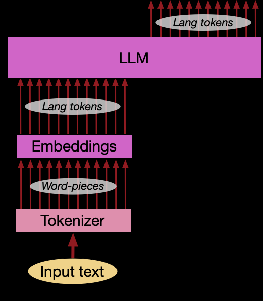
In a VLM architecture, the processor is usually a composite component that includes:

Tokenizer: for the text part
Image processor / feature extractor: for the image part This design allows a processor to handle multimodal inputs (text + images) in one place.

In a plain LLM, you only tokenize text. Here, we also need to create placeholders for image tokens within the token sequence, so the LLM decoder can replace those placeholders with image embeddings at runtime. So we define a special component that takes a user text prompt and an image, preprocesses the image (resize, normalize, etc.), and constructs text tokens that include image-token placeholders.

[!note] The Gemma tokenizer doesn’t come with special tokens for images, but PaliGemma can do multimodal autoregressive generation and also handle segmentation and detection. The key is that it expands the vocabulary. In the code below, it adds 1024 loc tokens for detection and 108 seg tokens for segmentation:

EXTRA_TOKENS = [
	f"<loc{i:04d}>" for i in range(1024) # left-pad with zeros; fixed field width; formatted as a decimal integer
]  # These tokens are used for object detection (bounding boxes)
EXTRA_TOKENS += [
	f"<seg{i:03d}>" for i in range(128)
]  # These tokens are used for object segmentation
tokenizer.add_tokens(EXTRA_TOKENS)

Tokenizer extension This is out of scope here; see the Hugging Face blog $^{[1]}$ for details.

We add an image token placeholder to the tokenizer; it will later be replaced by the embeddings extracted by the vision encoder.

In the parameters below:

num_image_token means how many consecutive <image> placeholders represent a single image.

class PaliGemmaProcessor:
 
    IMAGE_TOKEN = "<image>"
 
    def __init__(self, tokenizer, num_image_tokens: int, image_size: int):
        super().__init__()
 
        self.image_seq_length = num_image_tokens
        self.image_size = image_size
			# tokenizer.add_tokens(EXTRA_TOKENS)
        # Tokenizer described here: https://github.com/google-research/big_vision/blob/main/big_vision/configs/proj/paligemma/README.md#tokenizer
        tokens_to_add = {"additional_special_tokens": [self.IMAGE_TOKEN]}
        tokenizer.add_special_tokens(tokens_to_add)
        self.image_token_id = tokenizer.convert_tokens_to_ids(self.IMAGE_TOKEN)
        # We will add the BOS and EOS tokens ourselves
        tokenizer.add_bos_token = False
        tokenizer.add_eos_token = False
 
        self.tokenizer = tokenizer

Next, we’ll see how PaliGemmaProcessor adds the <image> placeholder into the tokenizer. When the model runs, the sequence positions occupied by these placeholders become the key “connection points” where image embeddings (from the vision tower) interact with the text sequence.

In the definition below, num_image_tokens specifies how many consecutive <image> placeholders represent one image. For example, if it’s set to 256, the input sequence fed to the language model will contain 256 <image> markers, giving the model enough “bandwidth” to integrate and understand the image.

    def __call__(
        self,
        text: List[str],            # input text prompt
        images: List[Image.Image],  # input PIL.Image
        # standard tokenizer padding and truncation strategies
        padding: str = "longest",
        truncation: bool = True,
    ) -> dict:
        assert len(images) == 1 and len(text) == 1, f"Received {len(images)} images for {len(text)} prompts." # only implements one image–text pair here
 
        pixel_values = process_images(
            images,
            size=(self.image_size, self.image_size),
            resample=Image.Resampling.BICUBIC,  # bicubic resampling preserves more detail/texture when resizing
            rescale_factor=1 / 255.0,           # rescale pixels to [0, 1]
            image_mean=IMAGENET_STANDARD_MEAN,  # standard mean (roughly [0.5, 0.5, 0.5]) 
            image_std=IMAGENET_STANDARD_STD,    # standard std (roughly [0.5, 0.5, 0.5])
        )
        # This will map pixel values to [-1, 1]
        # Convert the list of numpy arrays to a single numpy array with shape [Batch_Size, Channel, Height, Width]
        pixel_values = np.stack(pixel_values, axis=0) # stack into a batch
        # Convert the numpy array to a PyTorch tensor
        pixel_values = torch.tensor(pixel_values)

The image preprocessing pipeline:

   Image (PIL.Image) → resize → NumPy array → rescale (0–1) → normalize (mean/std) → transpose channel dim → PyTorch tensor

[!IMPORTANT] Constructing a VLM-specific input sequence is not just “string concatenation”—it builds an input that strictly follows the format used in pretraining. Any deviation (e.g., missing \n, wrong bos_token placement) can cause the model to misunderstand the prompt:

def add_image_tokens_to_prompt(prefix_prompt, bos_token, image_seq_len, image_token):
	# The trailing '\n' is critical for aligning with the training data format
	return f"{image_token * image_seq_len}{bos_token}{prefix_prompt}\n"

        # Prepend a `self.image_seq_length` number of image tokens to the prompt
        input_strings = [
            add_image_tokens_to_prompt(
                prefix_prompt=prompt,
                bos_token=self.tokenizer.bos_token,
                image_seq_len=self.image_seq_length, # number of <image> placeholders
                image_token=self.IMAGE_TOKEN,        # "<image>" string
            )
            for prompt in text
        ]

Then it goes through the tokenizer for the final conversion:

        # Convert the string sequence containing <image> placeholders into model-readable input_ids and attention_mask
        inputs = self.tokenizer(
            input_strings,
            return_tensors="pt",
            padding=padding,
            truncation=truncation,
        )
		# Return a dict containing the processed image tensor and the text token sequence
        return_data = {"pixel_values": pixel_values, **inputs}
 
        return return_data```
 
To make it easier to visualize the final form, here’s an example$^{[2]}$:
 
```python
from transformers.utils.attention_visualizer import AttentionMaskVisualizer
 
visualizer = AttentionMaskVisualizer("google/paligemma2-3b-mix-224")
visualizer("<img> What is in this image?")

Attention visualization

The yellow tokens in the figure are <image>.

Prefix-LM Masking

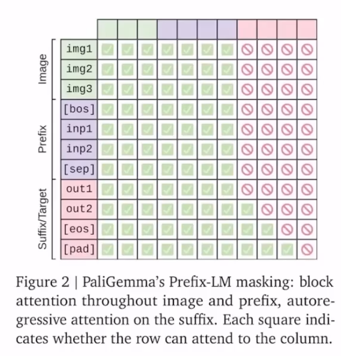
This work uses a prefix-LM masking strategy. That means the image tokens and the “prefix” (the task instruction prompt) use full (bidirectional) attention, so image tokens can “see” the task. A [sep] token (here it’s actually \n) separates them from the suffix. The “suffix” (the answer) is then generated autoregressively. Their ablations show this works better than applying autoregressive masking to the prefix or to the image tokens.

PaliGemma first forms a unified understanding of the image plus the input prompt (the prefix, i.e. the task instruction about the image). Then, like writing an essay, it generates the answer token by token, autoregressively (the suffix).

Prefix-LM masking strategy

LLM Decoder

The LLM’s workflow is shown below $^{[4]}$ (from a Groundlight.ai blog):

LLM workflow: text → tokens → embeddings

> Text → Tokens → Embeddings (features)

LLM workflow: embeddings → tokens → text

> Embeddings (features) → Tokens → Text

And below is the VLM workflow. As mentioned earlier, the preprocessor typically includes both the tokenizer and the image processor.

VLM workflow

class PaliGemmaForConditionalGeneration(nn.Module):
    def __init__(self, config: PaliGemmaConfig):
        super().__init__()
        self.config = config
        self.vision_tower = SiglipVisionModel(config.vision_config)
        self.multi_modal_projector = PaliGemmaMultiModalProjector(config)
        self.vocab_size = config.vocab_size
 
        language_model = GemmaForCausalLM(config.text_config)
        self.language_model = language_model
 
        self.pad_token_id = self.config.pad_token_id if self.config.pad_token_id is not None else -1
 
	# weight tying
    def tie_weights(self):
        return self.language_model.tie_weights()

[!note] One thing worth calling out: the embedding layer and the final linear layer that produces logits are basically inverses. The embedding layer maps token IDs to embeddings; the final linear layer maps contextual embeddings back to vocab-sized logits. Some models use a technique called weight tying, where these two layers share parameters to reduce total parameter count (since vocab size is large, this can save ~10%).

In forward, we first get embeddings for all input tokens, including the <image> placeholders. But those placeholder embeddings are not the real image features, so we’ll replace them later with the correct embeddings.

Screenshot 2025-05-21 at 16.10.46

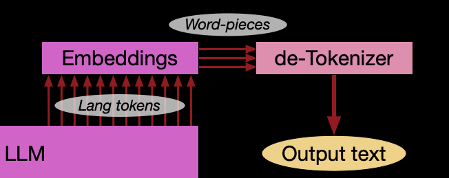
This figure visualizes patch tokens: after the VLM vision stack turns an image into feature vectors, it finds the closest text tokens in the language model’s vocabulary and shows their association strengths. That “poor” is a bit of a vibe killer…

def forward(
        self,
        input_ids: torch.LongTensor = None,
        pixel_values: torch.FloatTensor = None,
        attention_mask: Optional[torch.Tensor] = None,
        kv_cache: Optional[KVCache] = None,
    ) -> Tuple:
 
        # Make sure the input is right-padded
        assert torch.all(attention_mask == 1), "The input cannot be padded"
 
        # 1. Extra the input embeddings
        # shape: (Batch_Size, Seq_Len, Hidden_Size)
        inputs_embeds = self.language_model.get_input_embeddings()(input_ids)

The image patch tokens are encoded by the Vision Tower (SigLip) into patch embeddings:

        # 2. Merge text and images
        # [Batch_Size, Channels, Height, Width] -> [Batch_Size, Num_Patches, Embed_Dim]
        selected_image_feature = self.vision_tower(pixel_values.to(inputs_embeds.dtype))

[!tip] LLM embedding layer shape: (vocab_size, embedding_dim)

After SigLip, these image tokens are still in SigLip’s vector space, unrelated to the LLM’s text-token space. For SigLip they’re 768-dimensional vectors, while the Gemma LLM here uses 2048-dimensional vectors (hidden_size). So the most important part of the VLM is the projection layer below, which maps image patch vectors into the LLM’s text-token space.

		# [Batch_Size, Num_Patches, Embed_Dim] -> [Batch_Size, Num_Patches, Hidden_Size]
		image_features = self.multi_modal_projector(selected_image_feature)

The projector is just a linear layer:

class PaliGemmaMultiModalProjector(nn.Module):
    def __init__(self, config: PaliGemmaConfig):
        super().__init__()
        self.linear = nn.Linear(config.vision_config.hidden_size, config.vision_config.projection_dim, bias=True)
 
    def forward(self, image_features):
        # [Batch_Size, Num_Patches, Embed_Dim] -> [Batch_Size, Num_Patches, Projection_Dim]
        hidden_states = self.linear(image_features)
        return hidden_states

Now look at _merge_input_ids_with_image_features: the image mask and text mask are the key mechanisms that identify and distinguish different token types in the input sequence.

        # 3. Merge the embeddings of the text tokens and the image tokens
        inputs_embeds, attention_mask, position_ids = self._merge_input_ids_with_image_features(image_features, inputs_embeds, input_ids, attention_mask, kv_cache)

The Image Mask marks all image-token positions in the input sequence (True). It checks positions in input_ids where the value equals image_token_index (see added_tokens.json). Only at those positions does the model insert image features from the vision tower:

# Shape: [Batch_Size, Seq_Len]. True for image tokens
image_mask = input_ids == self.config.image_token_index # "<image>": 257152

The Text Mask marks all text-token positions (True). It is computed by selecting positions that are neither image tokens nor padding tokens. At those positions, the model inserts the text token embeddings:

# Shape: [Batch_Size, Seq_Len]. True for text tokens
text_mask = (input_ids != self.config.image_token_index) & (input_ids != self.pad_token_id)

Suppose the input sequence is: <image><image><image><bos>Describe this image. The image is processed into 3 patch embeddings, and the text is tokenized into text-token embeddings. We build the image/text masks and then expand them over the embedding dimension so they can be used to selectively fill the embedding tensor:

text_mask_expanded = text_mask.unsqueeze(-1).expand(-1, -1, embed_dim)
image_mask_expanded = image_mask.unsqueeze(-1).expand(-1, -1, embed_dim)

Then we apply the masks. We use masked_scatter for image embeddings because image features and the final embedding sequence have different lengths, so we can’t directly use torch.where:

# Place text embeddings
final_embedding = torch.where(text_mask_expanded, inputs_embeds, final_embedding)
 
# Place image embeddings
final_embedding = final_embedding.masked_scatter(image_mask_expanded, scaled_image_features)

Finally, we feed the result into the language model:

		# 4. Feed into the language model
        outputs = self.language_model(
            attention_mask=attention_mask,
            position_ids=position_ids,
            inputs_embeds=inputs_embeds,
            kv_cache=kv_cache,
        )
 
        return outputs

We then get the final logits (wrapped in a dict that may also include a KV cache):

class GemmaForCausalLM(nn.Module):
    # ... (other code) ...
 
    def forward(
        self,
        attention_mask: Optional[torch.Tensor] = None,
        position_ids: Optional[torch.LongTensor] = None,
        inputs_embeds: Optional[torch.FloatTensor] = None,
        kv_cache: Optional[KVCache] = None,
    ) -> Tuple:
 
        # ... (forward pass) ...
        outputs = self.model( # self.model is GemmaModel
            attention_mask=attention_mask,
            position_ids=position_ids,
            inputs_embeds=inputs_embeds,
            kv_cache=kv_cache,
        )
 
        hidden_states = outputs # final hidden state from GemmaModel
        logits = self.lm_head(hidden_states) # lm_head is a linear layer with output dim = vocab size
        logits = logits.float()
 
        return_data = {
            "logits": logits,
        }
 
        if kv_cache is not None:
            # Return the updated cache
            return_data["kv_cache"] = kv_cache
 
        return return_data

Future Directions

How can VLMs use image information more effectively, instead of ignoring the image and focusing only on text?
VLM + RL: improve reasoning over visual information for visual reasoning tasks—and improve interpretability.