LoRA in PyTorch

This article is a summary of my learning from GitHub - hkproj/pytorch-lora.

I’ve used the peft library for LoRA fine-tuning many times and understood the general principles, but I had never implemented it from scratch. This course content really hit the spot for me. ~~Classic ADHD: can’t rest until I’ve fully digested the knowledge.~~

Fine-Tuning

Object: Pre-trained models. Purpose: Learn from domain-specific or task-specific datasets to better adapt to particular application scenarios. Challenges: Full-parameter fine-tuning has high computational costs, model weights and optimizer states require massive VRAM, checkpoints take up large disk space, and switching between multiple fine-tuned models is inconvenient.

LoRA

LoRA (Low-Rank Adaptation) is a method of PEFT (Parameter-Efficient Fine-Tuning).

One of the core ideas behind LoRA is that many weights in the original weight matrix W may not be directly relevant to a specific fine-tuning task. Therefore, LoRA assumes that weight updates can be approximated by a low-rank matrix, meaning only a small number of parameter adjustments are sufficient to adapt to new tasks.

What is Rank?

Just as RGB primary colors can combine to create most colors, linearly independent vectors in a matrix’s column (or row) vectors can generate its column (or row) space. The primary colors can be seen as “basis vectors” of the color space, and the rank of a matrix is the number of basis vectors in its column (or row) space. The higher the rank, the richer the “colors” (vectors) the matrix can express.

Just as we can approximate a color image with grayscale (reducing color dimensions), low-rank approximation can be used to compress matrix information.

Motivation and Principle

See the original paper for details: LoRA: Low-Rank Adaptation of Large Language Models

Low-Rank Structure of Pre-trained Models: Pre-trained language models have a low “intrinsic dimension”; they can still learn effectively even when projected randomly onto a smaller subspace. This suggests that fine-tuning doesn’t require updating all parameters (ignoring bias); many can be expressed as combinations of others, making the model “rank deficient.”
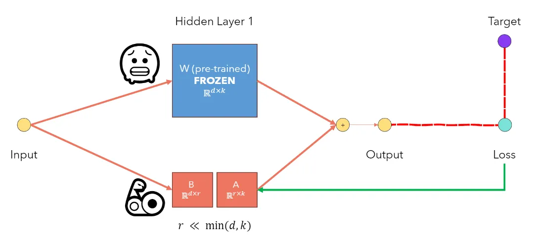
Low-Rank Update Hypothesis: Based on this finding, the authors hypothesized that weight updates also exhibit low-rank characteristics. During training, the pre-trained weight matrix W0 is frozen, and the update matrix ΔW is represented as the product of two low-rank matrices BA, where B and A are trainable matrices with rank r much smaller than d and k.
Formula Derivation: The updated weight matrix is expressed as $W_0 + \Delta$ and used in the forward pass as $h = W_0x + BAx$ . W0 remains frozen, while A and B are updated via gradients during backpropagation.

LoRA forward

Parameter Calculation

The original weight matrix W has $d \times k$ parameters. Let $d = 1000, k = 5000$ , resulting in $5,000,000$ parameters.
With LoRA, additional parameters come from matrices A and B. Their parameter count is: $p = (d \times r) + (r \times k)$ .

Typically $r$ is very small. For $r = 1$ :

p = (1000 \times 1) + (1 \times 5000) = 1000 + 5000 = 6000

This reduces the parameter count by 99.88%, drastically lowering fine-tuning computation costs, storage requirements, and model switching difficulty (only re-loading two low-rank matrices).

SVD

As mentioned, LoRA uses two low-rank matrices to represent massive parameter matrices. SVD (Singular Value Decomposition) is a common matrix decomposition method that splits a matrix into three sub-matrices:

W = U \Sigma V^T

import torch
import numpy as np
_ = torch.manual_seed(0)
 
d, k = 10, 10
W_rank = 2
W = torch.randn(d,W_rank) @ torch.randn(W_rank,k)
 
W_rank = np.linalg.matrix_rank(W) 
print(f'Rank of W: {W_rank}')
print(f"{W_rank=}")

Multiplying $10\times2$ and $2\times10$ matrices results in a $10 \times 10$ matrix W with a maximum rank of 2.

# Perform SVD on W (W = UxSxV^T)
U, S, V = torch.svd(W)
 
# For rank-r factorization, keep only the first r singular values (and corresponding columns of U and V)
U_r = U[:, :W_rank]
S_r = torch.diag(S[:W_rank])
V_r = V[:, :W_rank].t()  # Transpose V_r to get the right dimensions
 
# Compute B = U_r * S_r and A = V_r
B = U_r @ S_r
A = V_r
print(f'Shape of B: {B.shape}')
print(f'Shape of A: {A.shape}')

torch.svd(W) performs Singular Value Decomposition (SVD) on matrix W, yielding three matrices U, S, and V such that $W = U \cdot S \cdot V^T$ .

U: An orthogonal matrix whose columns are the left-singular vectors of W, dimension $d \times d$ .
S: A vector (the non-zero singular values on the diagonal of the diagonal matrix) containing the singular values of W, dimension $d$ .
V: An orthogonal matrix whose columns are the right-singular vectors of W, dimension $k \times k$ .

Retaining the first r singular values for low-rank approximation:

U_r = U[:, :W_rank]
S_r = torch.diag(S[:W_rank]) # Diagonal matrix of singular values
V_r = V[:, :W_rank].t()

Computing low-rank approximation:

B = U_r @ S_r
A = V_r

y: Result using the original matrix W. Multiplying $W$ ( $d \times k$ ) by $x$ ( $k \times 1$ ) takes $O(d \cdot k)$ operations.
y': Result using the reconstructed matrix $B \cdot A$ .
1. Calculate $A \cdot x$ ( $A$ is $r \times k$ ): $O(r \cdot k)$ operations.
2. Calculate $B \cdot (A \cdot x)$ ( $B$ is $d \times r$ , $A \cdot x$ is $r \times 1$ ): $O(d \cdot r)$ operations.

# Generate random bias and input
bias = torch.randn(d)
x = torch.randn(d)
 
# Compute y = Wx + bias
y = W @ x + bias
 
# Compute y' = (B*A)x + bias
y_prime = (B @ A) @ x + bias
 
# Check if the two results are approximately equal
if torch.allclose(y, y_prime, rtol=1e-05, atol=1e-08):
    print("y and y' are approximately equal.")
else:
    print("y and y' are not equal.")

Direct use of $W$ : Complexity $O(d \cdot k)$ .
Use of $B \cdot A$ : Total complexity $O(r \cdot k) + O(d \cdot r) = O(r \cdot (k + d))$ .

LoRA concept

$10\times10$ vs $2\times(10+10)$

LoRA isn’t strictly SVD; it uses trainable low-rank matrices A and B for dynamic weight adaptation.

Fine-Tuning LoRA for Classification

In an MNIST digit classification task, if a specific digit is poorly recognized, we can fine-tune it.

To showcase LoRA, let’s use a “sledgehammer to crack a nut” by defining a model far more complex than needed.

# Create an overly expensive neural network to classify MNIST digits
# Money is no object, so I don't care about efficiency
class RichBoyNet(nn.Module):
    def __init__(self, hidden_size_1=1000, hidden_size_2=2000):
        super(RichBoyNet,self).__init__()
        self.linear1 = nn.Linear(28*28, hidden_size_1) 
        self.linear2 = nn.Linear(hidden_size_1, hidden_size_2) 
        self.linear3 = nn.Linear(hidden_size_2, 10)
        self.relu = nn.ReLU()
 
    def forward(self, img):
        x = img.view(-1, 28*28)
        x = self.relu(self.linear1(x))
        x = self.relu(self.linear2(x))
        x = self.linear3(x)
        return x
 
net = RichBoyNet().to(device)

Let’s look at the parameter count.

LoRA verification

Train for one epoch and save original weights to prove LoRA won’t modify them.

train(train_loader, net, epochs=1)

Identify the poorly recognized digit:

Parametrization

We’ll choose “9” for fine-tuning.

Defining LoRA Parametrization

The forward function takes original_weights and returns a new weight matrix with the LoRA adaptation term added. During forward passes, the linear layer uses this new matrix.

class LoRAParametrization(nn.Module):
    def __init__(self, features_in, features_out, rank=1, alpha=1, device='cpu'):
        super().__init__()
        # A is Gaussian, B is zero, ensuring ΔW = BA starts as zero
        self.lora_A = nn.Parameter(torch.zeros((rank,features_out)).to(device))
        self.lora_B = nn.Parameter(torch.zeros((features_in, rank)).to(device))
        nn.init.normal_(self.lora_A, mean=0, std=1)
        
        # Scaling factor α/r simplifies hyperparameter tuning (Paper 4.1)
        self.scale = alpha / rank
        self.enabled = True
 
    def forward(self, original_weights):
        if self.enabled:
            # Return W + (B*A)*scale
            return original_weights + torch.matmul(self.lora_B, self.lora_A).view(original_weights.shape) * self.scale
        else:
            return original_weights

Initializing $A$ as normal and $B$ as zero makes initial $\Delta W = 0$ . Scaling $\frac{\alpha}{r}$ helps stabilize learning across different ranks $r$ .

Applying LoRA Parametrization

PyTorch’s parametrization mechanism (see Official Docs) allows custom parameter transformations without changing model structure. PyTorch moves the original parameter (e.g., weight) to a special location and uses the parametrization function to generate the new parameter.

We use parametrize.register_parametrization to apply LoRA to the linear layers:

import torch.nn.utils.parametrize as parametrize
 
def linear_layer_parameterization(layer, device, rank=1, lora_alpha=1):
    # Apply parametrization only to weights, ignore bias
    features_in, features_out = layer.weight.shape
    return LoRAParametrization(
        features_in, features_out, rank=rank, alpha=lora_alpha, device=device
    )

Original weights move to net.linear1.parametrizations.weight.original.
net.linear1.weight is now computed via the LoRA forward function.

parametrize.register_parametrization(
    net.linear1, "weight", linear_layer_parameterization(net.linear1, device)
)
parametrize.register_parametrization(
    net.linear2, "weight", linear_layer_parameterization(net.linear2, device)
)
parametrize.register_parametrization(
    net.linear3, "weight", linear_layer_parameterization(net.linear3, device)
)
 
def enable_disable_lora(enabled=True):
    for layer in [net.linear1, net.linear2, net.linear3]:
        layer.parametrizations["weight"][0].enabled = enabled

Parameter Comparison

Calculating parameter changes after introducing LoRA:

total_parameters_lora = 0
total_parameters_non_lora = 0
for index, layer in enumerate([net.linear1, net.linear2, net.linear3]):
    total_parameters_lora += layer.parametrizations["weight"][0].lora_A.nelement() + layer.parametrizations["weight"][0].lora_B.nelement()
    total_parameters_non_lora += layer.weight.nelement() + layer.bias.nelement()
    print(
        f'Layer {index+1}: W: {layer.weight.shape} + B: {layer.bias.shape} + Lora_A: {layer.parametrizations["weight"][0].lora_A.shape} + Lora_B: {layer.parametrizations["weight"][0].lora_B.shape}'
    )
# The non-LoRA parameters count must match the original network
assert total_parameters_non_lora == total_parameters_original
print(f'Total number of parameters (original): {total_parameters_non_lora:,}')
print(f'Total number of parameters (original + LoRA): {total_parameters_lora + total_parameters_non_lora:,}')
print(f'Parameters introduced by LoRA: {total_parameters_lora:,}')
parameters_incremment = (total_parameters_lora / total_parameters_non_lora) * 100
print(f'Parameters increment: {parameters_incremment:.3f}%')

LoRA results

LoRA introduces minimal parameters (~0.242%) yet enables effective fine-tuning.

Freezing non-LoRA Parameters

We only want to adjust LoRA-introduced parameters, keeping original weights frozen.

# Freeze the non-LoRA parameters
for name, param in net.named_parameters():
    if 'lora' not in name:
        print(f'Freezing non-LoRA parameter {name}')
        param.requires_grad = False

LoRA cover

Selecting the Target Dataset

To improve recognition of digit 9, we fine-tune using only digit 9 samples from MNIST.

# Keep only digit 9 samples
mnist_trainset = datasets.MNIST(root='./data', train=True, download=True, transform=transform)
digit_9_indices = mnist_trainset.targets == 9
mnist_trainset.data = mnist_trainset.data[digit_9_indices]
mnist_trainset.targets = mnist_trainset.targets[digit_9_indices]
 
# Create data loader
train_loader = torch.utils.data.DataLoader(mnist_trainset, batch_size=10, shuffle=True)

Fine-Tuning the Model

With original weights frozen, we fine-tune on digit 9 data for only 100 batches to save time.

# Fine-tune model for 100 batches
train(train_loader, net, epochs=1, total_iterations_limit=100)

Verifying Original Weights

Ensure original weights remain unchanged.

assert torch.all(net.linear1.parametrizations.weight.original == original_weights['linear1.weight'])
assert torch.all(net.linear2.parametrizations.weight.original == original_weights['linear2.weight'])
assert torch.all(net.linear3.parametrizations.weight.original == original_weights['linear3.weight'])
 
enable_disable_lora(enabled=True)
# New linear1.weight uses LoRAParametrization forward pass
# Original weights stay in net.linear1.parametrizations.weight.original
assert torch.equal(net.linear1.weight, net.linear1.parametrizations.weight.original + (net.linear1.parametrizations.weight[0].lora_B @ net.linear1.parametrizations.weight[0].lora_A) * net.linear1.parametrizations.weight[0].scale)
 
enable_disable_lora(enabled=False)
# Disabling LoRA restores original linear1.weight
assert torch.equal(net.linear1.weight, original_weights['linear1.weight'])

# Test with LoRA enabled
enable_disable_lora(enabled=True)
test()

Testing Model Performance

Comparing LoRA-enabled performance against the original model:

LoRA implementation

With LoRA, misidentifications of 9 dropped from 124 to 14. While overall accuracy (88.7%) is lower than without LoRA, performance on the specific target (digit 9) improved significantly without broad modification of other categories.