A First Look at Actor-Critic Methods

The Variance Problem

Policy Gradient methods have gained significant attention for their intuitiveness and effectiveness. We previously explored the Reinforce algorithm, which performs well in many tasks. However, the Reinforce method relies on Monte Carlo sampling to estimate returns, meaning we need data from an entire episode to calculate the return. This approach introduces a critical problem: high variance in policy gradient estimates.

Advantage estimation

The core of PG estimation lies in finding the direction of steepest return increase. In other words, we need to update the policy weights so that actions leading to higher returns have a higher probability of being selected in the future. Ideally, such updates will incrementally optimize the policy to obtain higher total returns.

However, when using Monte Carlo methods to estimate returns, because they rely on data from the entire episode to calculate the actual return (without estimation), the policy gradient estimate will have significant variance (unbiased but high variance). High variance means our gradient estimates are unstable, which can lead to slow training or even failure to converge. To obtain reliable gradient estimates, we might need a large number of samples, which is often costly in practical applications.

Reinforce variance

Randomness in the environment and policy can lead to vastly different returns from the same initial state, causing high variance. Therefore, returns starting from the same state can vary significantly across different episodes. Using a large number of trajectories can reduce variance and provide more accurate return estimates. However, large batch sizes reduce sample efficiency, hence the need for other mechanisms to reduce variance.

Advantage Actor-Critic (A2C)

Reducing Variance with Actor-Critic Methods

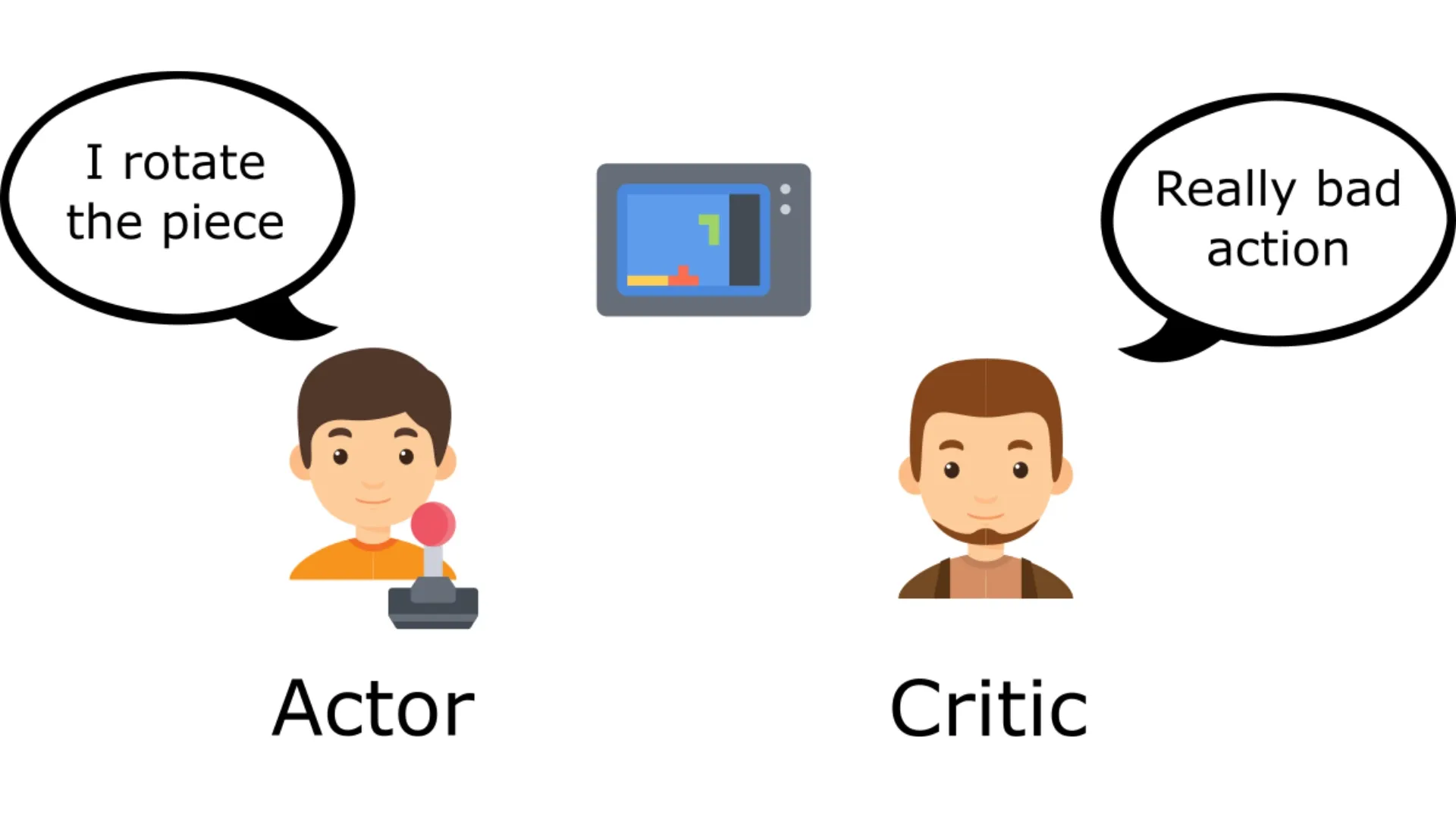
An intuitive takeaway from previous knowledge and the chapter introduction is that “if we combine Value-Based and Policy-Based methods, problems with variance and training will be optimized.” The Actor-Critic method is precisely such a hybrid architecture. Specifically:

Actor: Responsible for selecting actions, generating an action probability distribution based on the current policy.
Critic: Estimates the value function under the current policy, providing feedback on action selection.

Imagine you and your friend are both novice players. You are responsible for the controls (Actor), while your friend is responsible for observing and evaluating (Critic). Initially, neither of you knows much about the game. You operate somewhat blindly, while your friend is also figuring out how to evaluate your performance. Over time, you improve your skills through practice (Policy), while your friend learns to more accurately assess the quality of each action (Value).

Cover

You help each other and progress together: your actions provide the basis for your friend’s evaluation, and your friend’s feedback helps you adjust your strategy.

In other words, we learn two function approximations (neural networks):

A policy function that controls the agent (Actor): $\pi_\theta(s)$
A value function that measures the quality of actions and assists in policy optimization (Critic): $\hat{q}_w(s,a)$

Algorithm Workflow

At each time step $t$ , we obtain the current state $S_t$ from the environment and pass it as input to our Actor and Critic.
The Actor outputs an action $A_t$ based on the state.

A2C Algorithm

The Critic also takes the action as input and uses $S_t$ and $A_t$ to calculate the value of taking that action in that state: the Q-value.
The action $A_t$ is executed in the environment, resulting in a new state $S_{t+1}$ and a reward $R_{t+1}$ .
The Actor uses the $Q$ value to update its policy parameters.

Actor Critic Architecture

Training Code

The Actor uses the updated parameters to generate the next action $A_{t+1}$ given the new state $S_{t+1}$ .
The Critic then updates its value parameters.

TD Error

The Critic acts as a baseline for adjusting return estimates, thereby making gradient estimates more stable. The training process becomes smoother, convergence is faster, and the number of required samples is greatly reduced.

Adding Advantage (A2C)

Learning can be further stabilized by using the Advantage Function as the Critic instead of the action-value function.

Advantage: Let Good Actions Stand Out

The core idea is to evaluate your actions through two parts:

The immediate reward you receive and the value of the next state.
Your expectation of value in the current state.

Mathematically, we call this the Advantage:

A(s_t, a_t) = r_{t+1} + \gamma V(s_{t+1}) - V(s_t)

This expresses: in state $s_t$ , how much better is the action $a_t$ you made compared to your original expectation in state $s_t$ (the baseline expectation represented by $V(s_t)$ )?

If the actual reward and value of the future state $r_{t+1} + \gamma V(s_{t+1})$ is higher than your expectation for the current state $V(s_t)$ , then the action is good; if it’s lower, well… you can do better.

This advantage not only tells you if an action is good but also how good or how bad it is (relative to the baseline).

Policy Update

When we execute an action, the reward itself is not enough to guide policy improvement. The reward tells us whether an action is good or bad, but it doesn’t tell us exactly how good it is, or how much better than expected. So when improving the policy, focus on adjusting actions based on how much they exceed (or fall below) expectations. Now you can fine-tune the policy towards those actions that consistently perform better than the baseline.

This gives us the update formula:

\nabla_\theta J(\theta) \sim \sum_{t=0}^{T-1} \nabla_\theta \log \pi_\theta(a_t | s_t) A(s_t, a_t)

$\nabla_\theta \log \pi_\theta(a_t | s_t)$ : Represents the log gradient of the probability that policy $\pi_\theta$ selects action $a_t$ at each time step $t$ . This step helps us find how to change parameters $\theta$ to increase the likelihood of selecting $a_t$ under the current policy.
$A(s_t, a_t)$ : The advantage function of the action, telling us how much better or worse action $a_t$ is in state $s_t$ relative to the baseline.

In simple terms: the gradient of your policy $\pi_\theta$ is adjusted by the advantage $A(s_t, a_t)$ . You are updating your policy not just based on whether the action brought some reward, but based on how much the action exceeded expectations.

Better yet: you only need one neural network to predict the value function $V(s)$ .

Now Let’s Talk About TD Error

Calculating this advantage function is great, but there’s a beauty to online learning: you don’t have to wait until the end to update the policy. Enter Temporal Difference Error (TD Error):

\delta = r + \gamma V(s') - V(s)

The key point here is: TD Error is actually an online estimate of the advantage function. It tells you, at this very moment, whether your action made the future state better than you expected. This error $\delta$ directly reflects the concept of advantage:

If $\delta > 0$ : “Hey, this action is better than I thought!” (Positive advantage).
If $\delta < 0$ : “Hmm, I thought it would be better…” (Negative advantage).

This allows you to adjust your policy step-by-step without waiting for an entire episode to end. It’s an excellent strategy for improving efficiency.

Code Implementation

Actor-Critic Network Architecture

First, we need to build a neural network. This is a dual-headed network: one for the Actor (learning a policy to choose actions) and another for the Critic (estimating the value of states).

class ActorCritic(nn.Module):
    def __init__(self, num_inputs, num_actions, hidden_size, learning_rate=3e-4):
        super(ActorCritic, self).__init__()
 
        # Critic Network (Value Function Approximation)
        # This network predicts V(s), the value of state s
        self.critic_linear1 = nn.Linear(num_inputs, hidden_size)
        self.critic_linear2 = nn.Linear(hidden_size, 1)  # Value function is a scalar output
 
        # Actor Network (Policy Function Approximation)
        # This network predicts π(a|s), the probability of choosing action a in state s
        self.actor_linear1 = nn.Linear(num_inputs, hidden_size)
        self.actor_linear2 = nn.Linear(hidden_size, num_actions)  # Output probability distribution over all actions
    
    def forward(self, state):
        # Convert state to torch tensor and add a dimension for batch processing
        state = Variable(torch.from_numpy(state).float().unsqueeze(0))
        
        # Forward pass for Critic network
        value = F.relu(self.critic_linear1(state))
        value = self.critic_linear2(value)  # Output the value of state V(s)
        
        # Forward pass for Actor network
        policy_dist = F.relu(self.actor_linear1(state))
        policy_dist = F.softmax(self.actor_linear2(policy_dist), dim=1)  # Use softmax to convert raw values into action probabilities (policy)
        
        return value, policy_dist

Core Implementation of A2C Algorithm

Now for the heart of A2C: the main loop and update mechanism. In each episode, the agent runs for a certain number of steps in the environment, collecting a trajectory of states, actions, and rewards. At the end of each episode, the Actor (policy) and Critic (value function) are updated.

def a2c(env):
    # Get input and output dimensions from the environment
    num_inputs = env.observation_space.shape[0]
    num_outputs = env.action_space.n
    
    # Initialize Actor-Critic network
    actor_critic = ActorCritic(num_inputs, num_outputs, hidden_size)
    ac_optimizer = optim.Adam(actor_critic.parameters(), lr=learning_rate)
 
    # Data containers for tracking performance
    all_lengths = []  # Track length of each episode
    average_lengths = []  # Track average length of the last 10 episodes
    all_rewards = []  # Track cumulative rewards for each episode
    entropy_term = 0  # Encourage exploration
 
    # Loop through each episode
    for episode in range(max_episodes):
        log_probs = []  # Store log probabilities of actions
        values = []  # Store Critic's value estimates (V(s))
        rewards = []  # Store rewards received
 
        state = env.reset()  # Reset environment to start a new episode
        for steps in range(num_steps):
            # Forward pass through the network
            value, policy_dist = actor_critic.forward(state)
            value = value.detach().numpy()[0,0]  # Critic estimates the value of current state
            dist = policy_dist.detach().numpy()
            
            # Sample an action from the probability distribution
            action = np.random.choice(num_outputs, p=np.squeeze(dist))
            log_prob = torch.log(policy_dist.squeeze(0)[action])  # Record log probability of selected action
            entropy = -np.sum(np.mean(dist) * np.log(dist))  # Use entropy to measure exploration diversity
            new_state, reward, done, _ = env.step(action)  # Execute action, get reward and new state
 
            # Record trajectory data
            rewards.append(reward)
            values.append(value)
            log_probs.append(log_prob)
            entropy_term += entropy
            state = new_state  # Update to new state
            
            # If episode ends, record and exit loop
            if done or steps == num_steps-1:
                Qval, _ = actor_critic.forward(new_state)  # Value estimate for final state
                Qval = Qval.detach().numpy()[0,0]
                all_rewards.append(np.sum(rewards))  # Record total reward for episode
                all_lengths.append(steps)
                average_lengths.append(np.mean(all_lengths[-10:]))
                if episode % 10 == 0:
                    sys.stdout.write("episode: {}, reward: {}, total length: {}, average length: {} \n".format(
                        episode, np.sum(rewards), steps, average_lengths[-1]))
                break
 
        # Calculate Q-values (Critic's target values)
        Qvals = np.zeros_like(values)  # Initialize Q-value array
        for t in reversed(range(len(rewards))):
            Qval = rewards[t] + GAMMA * Qval  # Calculate Q-value using Bellman equation
            Qvals[t] = Qval
 
        Qvals = torch.FloatTensor(Qvals)
        log_probs = torch.stack(log_probs)
        
        # Calculate Advantage Function
        advantage = Qvals - values  # How much did the action exceed Critic's expectation?
 
        # Loss Functions
        actor_loss = (-log_probs * advantage).mean()  # Policy loss (encourage better-performing actions)
        critic_loss = 0.5 * advantage.pow(2).mean()  # Value function loss (minimize prediction error)
        ac_loss = actor_loss + critic_loss + 0.001 * entropy_term  # Total loss, including entropy incentive
 
        # Backpropagation and Optimization
        ac_optimizer.zero_grad()
        ac_loss.backward()
        ac_optimizer.step()

Actor update is based on policy gradient: we multiply the log probability of an action by its advantage. If an action performs better than expected (positive advantage), that action is encouraged.
Critic update is based on mean squared error: the Critic compares its predicted $V(s_t)$ with the actual return $Q_t$ and minimizes this difference.
entropy_term: Encourages exploration by introducing entropy, preventing the agent from converging too early to certain actions without sufficient exploration.

Summary

The core of A2C is guiding policy updates through the advantage function, while using TD Error for online learning to make the agent’s every move smarter and more efficient.

Advantage Function: Tells you not just if an action is good or bad, but how good it is relative to a baseline.
TD Error: A tool for real-time advantage calculation, helping you update the policy quickly and efficiently.

Asynchronous A2C (A3C)

A3C was proposed in DeepMind’s paper “Asynchronous Methods for Deep Reinforcement Learning”. Essentially, A3C is a parallelized version of A2C. Multiple parallel agents (worker threads) independently update a global value function in parallel environments, hence “asynchronous.” It is highly efficient on modern multi-core CPUs.

As seen before, A2C is the synchronous version of A3C, waiting for each participant to finish its experience segment before performing updates and averaging results. Its advantage is more efficient GPU utilization. As mentioned in OpenAI Baselines: ACKTR & A2C: Our synchronous A2C implementation outperforms our asynchronous implementation — we have not seen any evidence that the noise introduced by asynchrony provides any performance advantage. This A2C implementation is more cost-effective than A3C when using single-GPU machines and is faster than a CPU-only A3C implementation when using larger policies.