PPO Speedrun

Proximal Policy Optimization

We’ve finally reached one of the hottest RL algorithms in the NLP field in recent years.

In On-Policy algorithms, the policy used to collect data is the same as the policy being trained. The problem with this is that data must be discarded after a single use, requiring re-collection, which makes training very slow.

Intuition Behind PPO

The idea of PPO is to improve training stability by limiting the changes made to the policy in each training cycle: avoiding drastic policy updates.

This is based on two reasons:

• Empirical evidence in the field suggests that smaller policy updates are more likely to converge to an optimal solution.
• In policy updates, a step that is too large can lead to “falling off a cliff” (resulting in a bad policy) and take a long time to recover, or even never return to the original level.

Clipped Surrogate Objective Function

Review: Policy Objective Function

Our goal is to use gradient ascent (or the negative of gradient descent) to drive the agent toward behaviors that yield higher rewards and away from actions that might have negative effects.

1. $\log \pi_\theta(a_t | s_t)$: The log probability of choosing action $a_t$ given state $s_t$, representing the probability of taking this action under the current policy.
2. $A_t$: The Advantage function. If $A > 0$, the action is better than other possible actions in the current state; otherwise, it is worse.

However, classical PG methods have a problem: the choice of policy update step size is crucial.

• If the step size is too small, training will be very slow.
• If the step size is too large, there is too much volatility, potentially leading to instability.

Thus, PPO proposes a new solution, the Clipped Surrogate Objective Function, which clips the range of policy changes to ensure updates aren’t too aggressive, thereby maintaining training stability.

This new objective function is as follows:

The Ratio Function

A key part is the ratio function $r_t(\theta)$, representing the probability ratio of an action under the current policy versus the previous policy:

The ratio reflects the degree of deviation between the current and old policies:

• If $r_t(\theta) \in (0, 1)$, the probability of choosing that action has decreased under the current policy.
• If $r_t(\theta) > 1$, the action $a_t$ is more likely to be chosen than before.

Unclipped Part

The unclipped part of the formula is:

In the unclipped objective function, $r_t(\theta)$ is multiplied directly by the advantage value $\hat{A}_t$. If action $a_t$ is better under the current policy than the old one ($\hat{A}_t > 0$), we promote the action; otherwise, we weaken its influence. This is the standard direction for policy gradient optimization.

But as mentioned, unconstrained policy updates can lead to instability. If the ratio $r_t(\theta)$ is far greater than 1, the update will be too large, making convergence difficult.

This is where PPO introduces its clipping strategy to constrain the range of the ratio.

Clipped Part

Here we see the introduction of the $\min$ operation. When the ratio $r_t(\theta)$ exceeds the threshold $[1 - \epsilon, 1 + \epsilon]$, the clipping operation limits the ratio to this range, preventing excessive updates.

The clipping function is:

This means if the ratio $r_t(\theta)$ falls outside the interval (typically $\epsilon = 0.2$ in the original paper), it is truncated to be between $[0.8, 1.2]$, ensuring stability. We take the minimum of the truncated and untruncated values, ensuring the final objective function isn’t overly optimistic but rather a more conservative estimate.

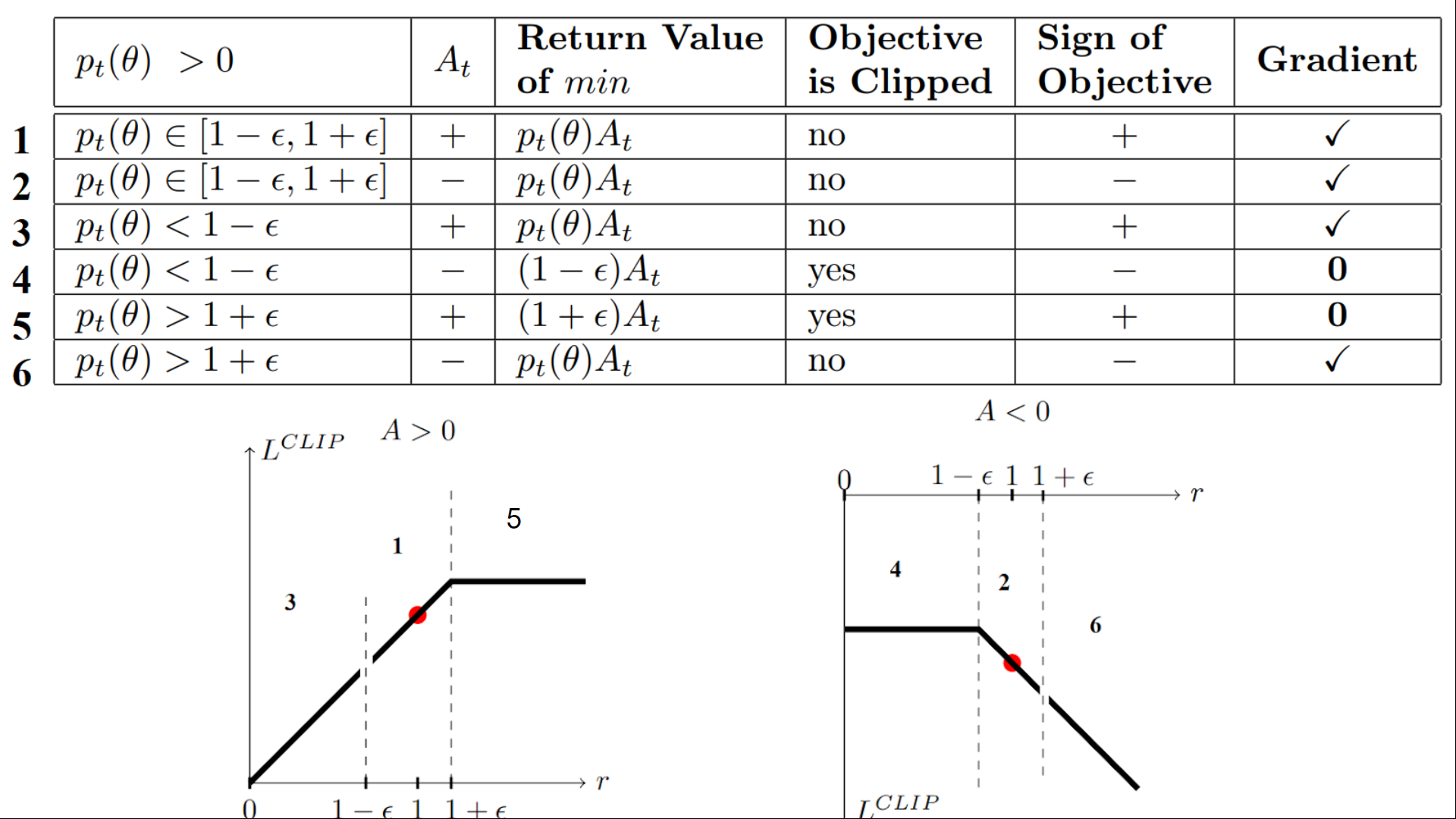
Visualization

Remember, we take the minimum of the clipped and unclipped targets.

Cases 1 and 2: Ratio Within Range

In these cases, no clipping occurs, and the policy updates based on whether $A_t$ is positive or negative. This is the ideal state for PPO.

• Case 1: $A_t > 0$ and $r_t(\theta) \in [1 - \epsilon, 1 + \epsilon]$

  • Positive advantage means the action was better than expected.
  • The ratio is within range, so the change isn’t large. We want to encourage this action, so no clipping.
  • Result: Positive objective; gradient updates further favor this action.

• Case 2: $A_t < 0$ and $r_t(\theta) \in [1 - \epsilon, 1 + \epsilon]$

  • Negative advantage means the action was worse than expected.
  • No clipping since the ratio is within range. We want to reduce the frequency of this action.
  • Result: Negative objective; gradient updates move the policy away from this action.

Cases 3 and 4: Ratio Below Range

Here the ratio indicates the current policy underestimates the probability of the action compared to the old policy.

• Case 3: $A_t > 0$ and $r_t(\theta) < 1 - \epsilon$

  • The action is good (positive advantage), but the new policy thinks it has a lower probability.
  • We do not clip because we want to increase the probability of this excellent action, allowing strong gradient-driven updates.
  • Result: Positive objective; gradient encourages the action.

• Case 4: $A_t < 0$ and $r_t(\theta) < 1 - \epsilon$

  • The action is bad (negative advantage), and the policy is already reducing its probability.
  • However, we clip because the probability is already below $1 - \epsilon$. Continuing to lower it might over-penalize and cause instability.
  • Result: Objective is clipped; gradient stops updating, and the action probability stays at the lower bound.

Cases 5 and 6: Ratio Above Range

In this scenario, the policy is overconfident in the action, meaning the new policy has made its execution probability too high.

• Case 5: $A_t > 0$ and $r_t(\theta) > 1 + \epsilon$

  • The action is good (positive advantage), but the new policy overestimates its probability.
  • We clip because we don’t want the policy to over-favor this action. Even with a positive $A_t$, we need to limit the update step size.
  • Result: Objective is clipped; gradient stops updating, limiting the magnitude of change.

• Case 6: $A_t < 0$ and $r_t(\theta) > 1 + \epsilon$

  • The action is bad, yet the policy has increased its probability. This is definitely not what we want.
  • The ratio is out of range, but we don’t clip. The negative objective allows the gradient to strongly push the policy away from this bad action.
  • Result: Negative objective; gradient pushes the policy away from the action.

Why is the Gradient Zero When Clipped?

When the ratio $r_t(\theta)$ is clipped to $1 - \epsilon$ or $1 + \epsilon$, the derivative is no longer that of $r_t(\theta) \times A_t$, but rather the derivative of $(1 - \epsilon)A_t$ or $(1 + \epsilon)A_t$, both of which are 0.

Summary

To summarize, PPO aims to limit the change between current and old policies using the Clipped Surrogate Objective. We remove the incentive for the ratio to move beyond the $[1 - \epsilon, 1 + \epsilon]$ interval because once it’s outside, the gradient becomes 0 and updates stop.

In the PPO update process, we only update the policy in two cases:

1. When the ratio $r_t(\theta)$ falls within $[1 - \epsilon, 1 + \epsilon]$.
2. When the ratio is outside the interval, but the advantage function pulls it back toward the interval.

Finally, the PPO Clipped Surrogate Objective Loss consists of three parts:

• Clipped Surrogate Objective function: Limits the range of policy updates.
• Value Loss Function: Minimizes the mean squared error of the value function.
• Entropy Bonus: Maintains sufficient exploration to prevent the policy from falling into local optima prematurely.

These three parts combine to ensure PPO can both stabilize policy updates and maintain sufficient exploration.

Code Implementation

Let’s understand the PPO implementation from a code perspective, focusing on the most critical parts of CleanRL’s ppo.py.

1. Policy and Value Network Structure

class Agent(nn.Module):
    def __init__(self, envs):
        super().__init__()
        # Critic network: Maps states to values (estimating how good a state is)
        self.critic = nn.Sequential(
            layer_init(nn.Linear(np.array(envs.single_observation_space.shape).prod(), 64)),
            nn.Tanh(),
            layer_init(nn.Linear(64, 64)),
            nn.Tanh(),
            layer_init(nn.Linear(64, 1), std=1.0), # Initialization of the last layer is key for stability
        )
        # Actor network: Maps states to action probabilities (the policy network)
        self.actor = nn.Sequential(
            layer_init(nn.Linear(np.array(envs.single_observation_space.shape).prod(), 64)),
            nn.Tanh(),
            layer_init(nn.Linear(64, 64)),
            nn.Tanh(),
            layer_init(nn.Linear(64, envs.single_action_space.n), std=0.01), # Small std ensures near-uniform initial policy
        )

This is a typical dual-network architecture:

• The actor outputs the action probability distribution.
• The critic predicts state values.
• Both use simple two-layer MLP structures (64-64).
• Orthogonal initialization helps with training stability.

2. GAE (Generalized Advantage Estimation) Implementation

# GAE calculation: Backward recurrence to compute advantages and returns
with torch.no_grad():
    next_value = agent.get_value(next_obs).reshape(1, -1)
    advantages = torch.zeros_like(rewards).to(device)
    lastgaelam = 0
    for t in reversed(range(args.num_steps)):
        # GAE (Generalized Advantage Estimation) elegant implementation
        # It can be understood as an exponentially weighted sum of TD errors
        delta = rewards[t] + args.gamma * nextvalues * nextnonterminal - values[t]
        advantages[t] = lastgaelam = delta + args.gamma * args.gae_lambda * nextnonterminal * lastgaelam
    returns = advantages + values  # Return = Advantage + Value estimate

This shows the recursive GAE calculation:

• TD errors (delta) are computed from back to front.
• These errors are accumulated using exponential weighting.
• Gamma and lambda hyperparameters control the bias-variance tradeoff of the value estimate.

3. Core PPO Loss Calculation

# PPO Core: Improving the policy while preventing excessive changes
_, newlogprob, entropy, newvalue = agent.get_action_and_value(b_obs[mb_inds], b_actions.long()[mb_inds])
ratio = (newlogprob - b_logprobs[mb_inds]).exp()  # Importance sampling ratio
 
# The famous PPO-Clip objective function
pg_loss1 = -mb_advantages * ratio
pg_loss2 = -mb_advantages * torch.clamp(ratio, 1 - args.clip_coef, 1 + args.clip_coef)
pg_loss = torch.max(pg_loss1, pg_loss2).mean()  # Pessimistic (worst-case) policy loss
 
# Value function loss also uses clipping to stay close to old predictions
if args.clip_vloss:
    v_loss_unclipped = (newvalue - b_returns[mb_inds]) ** 2
    v_clipped = b_values[mb_inds] + torch.clamp(
        newvalue - b_values[mb_inds],
        -args.clip_coef,
        args.clip_coef,
    )
    v_loss_clipped = (v_clipped - b_returns[mb_inds]) ** 2
    v_loss = 0.5 * torch.max(v_loss_unclipped, v_loss_clipped).mean()
 
# Combined loss: strategy loss, value loss, and entropy bonus for exploration
loss = pg_loss - args.ent_coef * entropy_loss + v_loss * args.vf_coef

This implements the three key components mentioned earlier:

• Clipped Surrogate Objective using max for truncation (since we are minimizing negative loss).
• Value function loss clipping (a feature of the OpenAI implementation).
• Entropy bonus to encourage exploration.

After a long delay due to platform IPFS issues, this post officially concludes the Hugging Face Deep RL series!