Let’s build AlphaZero

This article is a digestion and synthesis of resources like Sunrise: Understanding AlphaZero from Scratch, MCTS, Self-Play, UCB, various video tutorials, and code implementations.

Starting from the design principles of AlphaGo and diving deep into the core mechanisms of MCTS and Self-Play, we will reveal step-by-step how to build an AI Gomoku (Five-in-a-Row) system that can surpass human capabilities.

AlphaGo: From Imitation to Transcendence

The Evolutionary Path of AlphaGo

The number of possible positions in Go exceeds the number of atoms in the universe, making traditional exhaustive search methods completely obsolete. AlphaGo solved this problem through a phased approach: first learning from human knowledge, then continuously evolving through self-play.

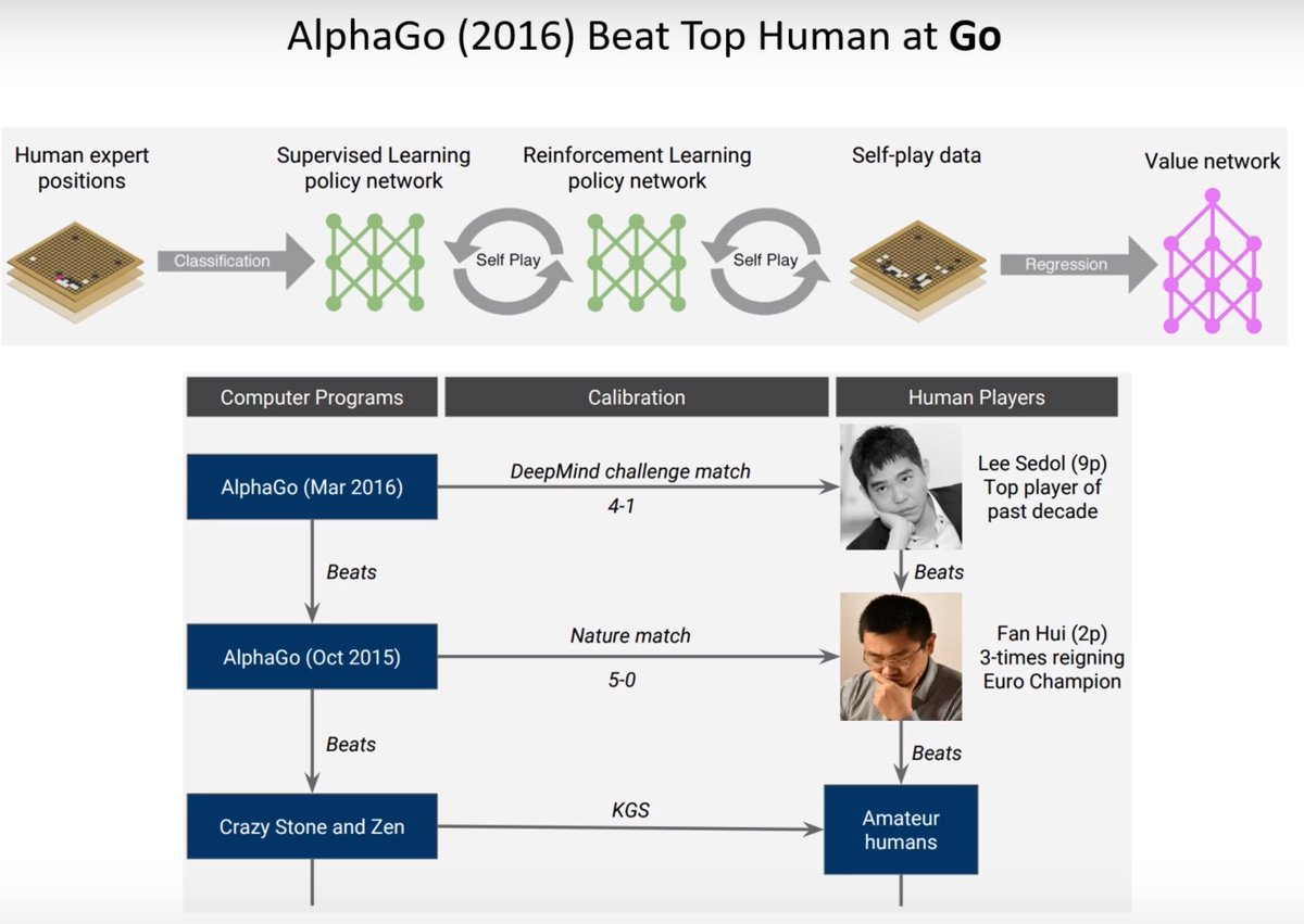
This evolutionary process can be divided into three layers:

1. Imitating human experts
2. Self-play improvement
3. Learning to evaluate board positions

Core Components

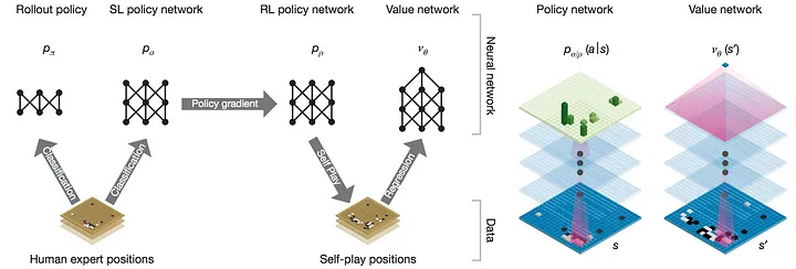
Rollout Policy

The lightweight policy network on the far left, used for rapid evaluation. It has lower accuracy but high computational efficiency.

SL Policy Network

The Supervised Learning policy network $P_{\sigma}$ learns to play by imitating human game records:

• Input: Board state
• Output: Probability distribution of next moves imitating human experts
• Training Data: 160,000 games, approximately 30 million moves

RL Policy Network

This is like when your skill reaches a certain level, you start reviewing your own games and playing against yourself to discover new tactics and deeper strategies. The RL network $P_{ ho}$ is initialized from the SL network. This network already far surpasses humans and can find many powerful strategies humans have never discovered.

• This phase generates a large amount of self-play data. The input is still the board state, and the output is the move strategy improved through reinforcement learning.
• Self-play is conducted against historical versions of the policy network $p_\pi$. The network adjusts parameters based on “winning” signals, using Policy Gradient to reinforce moves that lead to victory:
  $$\sum_{t} z(\tau) \log p(a_t \mid s_t; \rho)$$
  Where:
• $\tau$ is the game sequence $(s_0,a_0,s_1,a_1,...)$
• $z(\tau)$ is the win/loss label (positive for win, negative for loss)

Value Network

The value network $v_\theta$ learns to evaluate the board state; it can be a CNN:

• Training Goal: Minimize Mean Squared Error (MSE)
  $$\sum_{i} (z - v_\theta(s))^2$$
• $z$: Final win/loss outcome
• $v_\theta(s)$: Predicted winning probability

Supplemental Explanation

Relationship between $P_\rho$ and $v_\theta$:

• The policy network $P_\rho$ provides specific move probabilities to guide the search.
• The value network $v_\theta$ provides board evaluation, reducing unnecessary simulations in the search tree.
• Together, they allow MCTS to not only explore high-win-rate paths faster but also significantly improve the overall level of play.

AlphaGo’s MCTS Implementation

Selection Phase

Combines exploration and exploitation:

Where:

• $Q(s_t, a)$: Long-term return estimate
• $u(s_t, a)$: Exploration bonus
• $P(s_t, a)$: Prior probability from the policy network
• $N(s_t, a)$: Visit count

Simulation and Evaluation

In the original MCTS algorithm, the purpose of the Simulation phase is to conduct random play from a leaf node (a newly expanded node) using a fast rollout policy until the game ends, then obtaining a return based on the win or loss. This return is propagated back to the nodes in the search tree to update their value estimates (i.e., $Q(s, a)$).

While simple and direct, rollout policies are usually random or simple rules, leading to potentially poor simulation quality. Moreover, they only provide short-term information and don’t integrate well with global strategic evaluation.

AlphaGo, however, combines the Value Network $v_\theta$ with the rollout policy during the simulation phase. The Value Network provides more efficient leaf node estimation and global ability evaluation, while the rollout policy captures local short-term effects through fast simulation.

A hyperparameter $\lambda$ is used to balance $v_\theta(s_L)$ and $z_L$, considering both local simulation and global evaluation. Evaluation function:

Backpropagation

Update of node visit counts during $n$ MCTS iterations ($\mathbb{I}$ is the indicator function, 1 if visited):

Q-value update, i.e., the long-term expected return of executing action $a$ to node $s_t$:

Summary

1. Structural Innovation:

   • Policy network provides prior knowledge
   • Value network provides global evaluation
   • MCTS provides tactical verification

2. Training Innovation:

   • Starting from supervised learning
   • Surpassing the teacher through reinforcement learning
   • Self-play generates new knowledge

3. MCTS Improvements:

   • Using neural networks to guide the search
   • The Policy Network provides prior probabilities for exploration directions, and the Value Network improves the accuracy of leaf node evaluation.
   • This combination of value network and rollout evaluation not only reduces search width and depth but also significantly improves overall performance.
   • Efficient balance of exploration and exploitation.

This design enables AlphaGo to find efficient solutions in a vast search space, ultimately surpassing human levels.

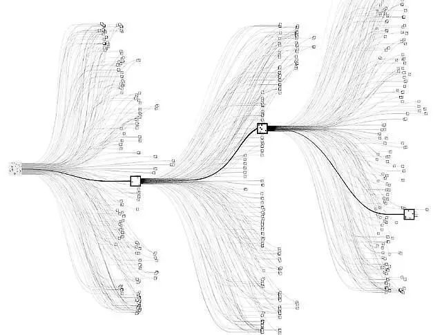
Heuristic Search and MCTS

MCTS is like an evolving explorer looking for the best path in a decision tree.

Core Idea

What is the essence of MCTS? Simply put, it’s a process of “learning while playing.” Imagine playing a brand-new board game:

• At first, you try all sorts of possible moves (exploration)
• Gradually, you discover that some moves work better (exploitation)
• You strike a balance between exploring new strategies and exploiting known good ones

This is exactly what MCTS does, just systematic and mathematical. It is a rollout algorithm that guides policy selection by accumulating value estimates from Monte Carlo simulations.

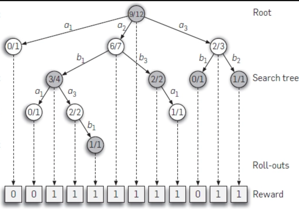
Algorithm Workflow

Monte Carlo Tree Search - YouTube - this teacher explains the MCTS process very well.

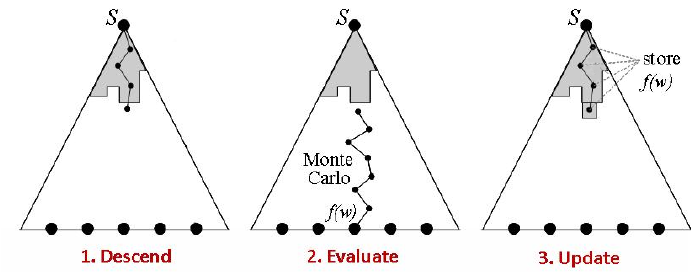
The elegance of MCTS lies in its four simple but powerful steps. I’ll introduce them using two ways of understanding, A and B:

1. Selection

   • A: Do you know how children learn? They are always oscillating between the known and the unknown. MCTS is the same: starting from the root node, it uses the UCB (Upper Confidence Bound) formula to weigh whether to choose a known good path or explore new possibilities.
   • B: Starting from the root node, a successor node is selected from the current node according to a specific policy. This policy is usually based on the tree’s search history, picking the most promising path. For example, at each node, we execute action $a$ according to the current policy $\pi(s)$ to balance exploration and exploitation, going deeper step by step.

2. Expansion

   • A: Like an explorer opening up new areas on a map, when we reach a leaf node, we expand downwards, creating new possibilities.
   • B: When a selected node still has unexplored child nodes, we expand a new node under this node according to the set of available actions. The purpose of this process is to increase the width of the decision tree, gradually generating possible decision paths. Through this expansion, we ensure the search covers more possible state-action pairs $(s,a)$.

3. Simulation

   • A: This is the most interesting part. Starting from the new node, we conduct an “imaginary” game until it ends. This is like chess players deducing in their minds: “If I go this way, and my opponent goes that way…”
   • B: Starting from the currently expanded node, a random simulation (rollout) is executed, sampling along the current policy $\pi(s)$ in the MDP environment until a terminal state is reached. This process provides a return estimate from the current node to the end, providing a numerical basis for the path’s quality.

4. Backpropagation

   • A: Finally, we return the results obtained along the path, updating the statistical information of each node. It’s like saying: “Hey, I tried this path, and it worked out okay (or not so well).”
   • B: After completing the simulation, the estimated return is backpropagated to all nodes passed through to update their values. This process accumulates historical return information, making future choices more precisely trend toward high-yield paths.

UCB1: The Perfect Balance of Exploration and Exploitation

The UCB1 formula deserves special mention as the soul of MCTS:

Let’s deconstruct it:

• $X̄ᵢ$ is the average reward (exploitation term)
• $\sqrt{(ln(N)/nᵢ)}$ is the measure of uncertainty (exploration term)
• $C$ is the exploration parameter

Like a good investment portfolio, you need to focus on known good opportunities while remaining open to new ones (exploration-exploitation trade-off).

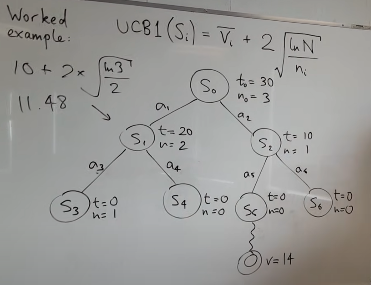
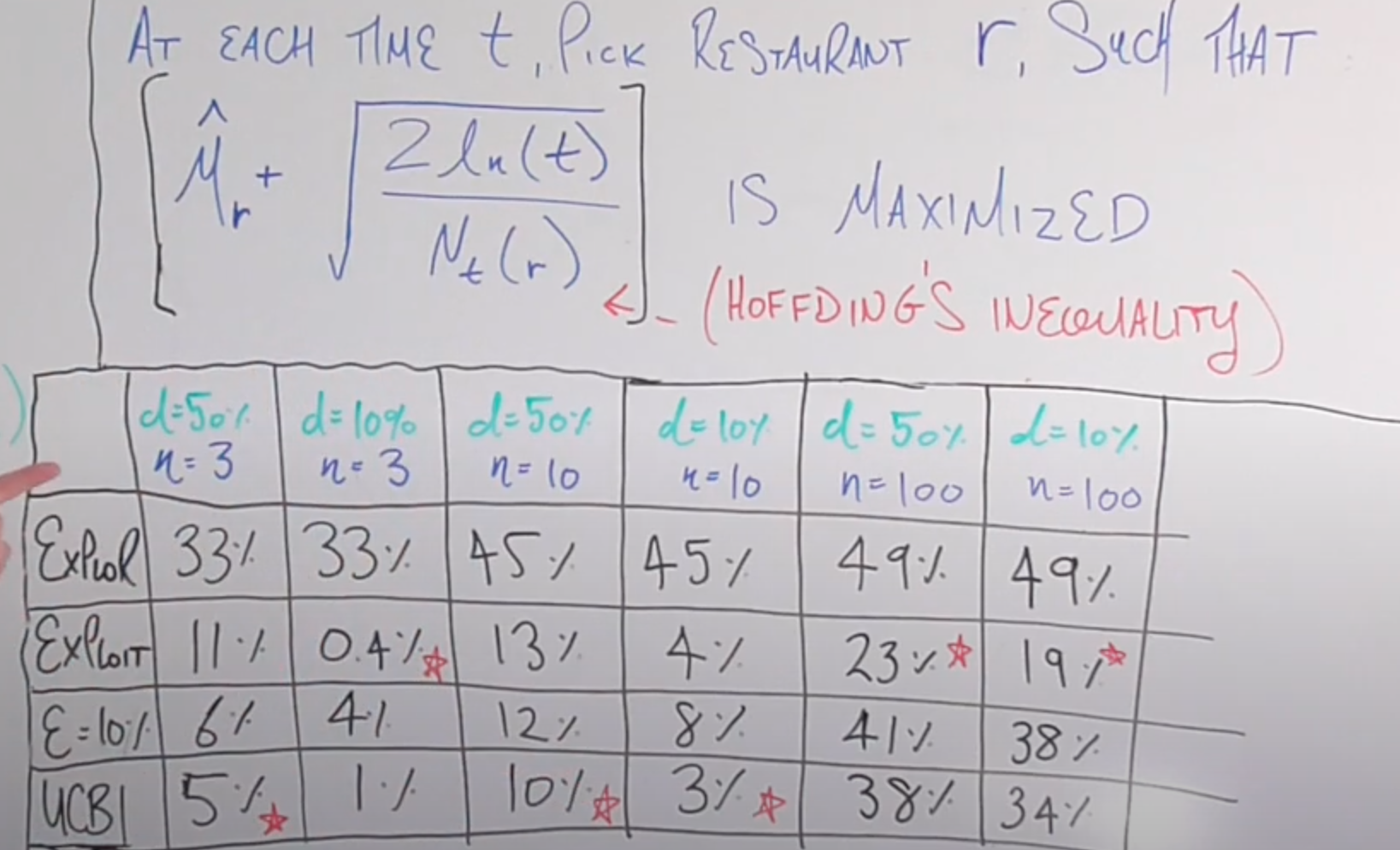
Best Multi-Armed Bandit Strategy? (feat: UCB Method) - This video explains the Multi-Armed Bandit and UCB Method very well. I’ll borrow the example used by this teacher:

A Foodie’s Attempt to Understand UCB

Imagine you’ve just arrived in a city with 100 restaurants to choose from, and you have 300 days. Every day you must choose a restaurant to dine at, hoping to eat the best food on average over those 300 days.

ε-greedy Policy: Simple but Not Smart Enough

This is like deciding with a roll of the dice:

• 90% of the time (ε=0.1): Go to the best known restaurant (exploitation)
• 10% of the time: Randomly try a new restaurant (exploration)

def epsilon_greedy(restaurants, ratings, epsilon=0.1):
    if random.random() < epsilon:
        return random.choice(restaurants)  # Exploration
    else:
        return restaurants[np.argmax(ratings)]  # Exploitation

The effect is:

• Exploration is completely random and might repeatedly visit restaurants known to be bad.
• The exploration ratio is fixed and won’t adjust over time.
• It doesn’t consider the number of visits.

UCB Policy: A Smarter Choice Trade-off

The meaning of the UCB formula in restaurant selection is as follows:

For example, consider the situation of two restaurants on day 100:

Restaurant A:

• 50 visits, average score 4.5
• UCB Score = $4.5 + 2×\sqrt{ln(100)/50} ≈ 4.5 + 0.6 = 5.1$

Restaurant B:

• 5 visits, average score 4.0
• UCB Score = $4.0 + 2×\sqrt{ln(100)/5} ≈ 4.0 + 1.9 = 5.9$

Although Restaurant B has a lower average score, because it has fewer visits and high uncertainty, UCB gives it a higher exploration bonus.

Code implementation:

class Restaurant:
    def __init__(self, name):
        self.name = name
        self.total_rating = 0
        self.visits = 0
        
def ucb_choice(restaurants, total_days, c=2):
    # Ensure each restaurant is visited at least once
    for r in restaurants:
        if r.visits == 0:
            return r
            
    # Use UCB formula to select a restaurant
    scores = []
    for r in restaurants:
        avg_rating = r.total_rating / r.visits
        exploration_term = c * math.sqrt(math.log(total_days) / r.visits)
        ucb_score = avg_rating + exploration_term
        scores.append(ucb_score)
        
    return restaurants[np.argmax(scores)]

Why is UCB Better?

1. Adaptive Exploration

   • Restaurants with fewer visits get higher exploration bonuses.
   • As total days increase, the exploration term gradually decreases for better exploitation.

2. Balanced Time Investment

   • You won’t waste too much time on obviously inferior restaurants.
   • You’ll reasonably allocate visits between restaurants with similar potential.

3. Theoretical Guarantees

   • Regret Bound (the gap from the optimal choice) grows logarithmically over time.
   • 300 days of exploration is enough to find the best few restaurants.

Back to MCTS:

Why is MCTS so Powerful?

• Efficiently Handles Combinatorial Explosion: MCTS doesn’t need to exhaustively search all possibilities like Minimax; it focuses on the most promising branches, allowing it to effectively handle problems with massive branching factors.
• Adaptive Search: MCTS dynamically adjusts its search strategy, allocating more resources to more promising areas, thereby finding good solutions faster.
• Balances Exploration and Exploitation: Through the UCB formula, MCTS balances exploring new possibilities with exploiting known good choices, avoiding getting stuck in local optima.
• No Domain Knowledge Required: MCTS doesn’t rely on domain-specific expertise, relying only on game rules and simulation results to learn, giving it broad applicability.
• Anytime Algorithm: MCTS can be interrupted at any time to return the current best solution, which is crucial for real-time applications.

AlphaZero: From MCTS to Self-Evolution

AlphaZero is a general reinforcement learning algorithm introduced by DeepMind after AlphaGo. It can learn from scratch through Self-Play and ultimately surpass professional levels without using human game records.

AlphaZero improves upon traditional MCTS by introducing Neural Networks to guide the search:

• Policy Priors: Uses a neural network to predict the prior probability of each action, making the search more efficient.
• Value Evaluation: At leaf nodes, it uses value predictions from the neural network instead of random simulations, reducing computational costs.

Let’s use Gomoku as an example to implement an AI that can learn this way. We’ll learn from and reference the excellent implementation in schinger/alphazero.py.

Game Environment Design

Before implementing AlphaZero, we first need to define the game environment.

Defining the Game Interface

In AlphaZero, the neural network receives the current board state and outputs a policy vector $\boldsymbol{P}$ representing the probability of each action, and a scalar value $v$ representing the predicted win rate for the current player.

To make MCTS and the neural network interact with games in a general way, we need to define a consistent game interface.

class GomokuGame:
    def __init__(self, n=15):
        self.n = n  # Board size, default 15x15
 
    def getInitBoard(self):
        """
        Returns the initial board state, with all positions empty.
        """
        b = Board(self.n)
        return np.array(b.pieces)
 
    def getBoardSize(self):
        """
        Returns the board dimensions, (n, n).
        """
        return (self.n, self.n)
 
    def getActionSize(self):
        """
        Returns the total number of actions, which is n * n since every square is a possible move.
        """
        return self.n * self.n
 
    def getNextState(self, board, player, action):
        """
        Executes an action and returns the next board state and next player.
 
        Parameters:
        - board: Current board state
        - player: Current player (1 or -1)
        - action: Current action, 0 ~ n*n-1
 
        Returns:
        - (next_board, next_player): Board and next player after the action
        """
        b = Board(self.n)
        b.pieces = np.copy(board)
        # Convert action to coordinates (x, y)
        move = (action // self.n, action % self.n)
        b.execute_move(move, player)
        return (b.pieces, -player)

• Unified Interface: Allows our MCTS and neural network to be reused across different games by only implementing the specific game logic.
• Board Representation: Uses a 2D array to represent the board, facilitating processing and visualization.

Core Algorithm Implementation

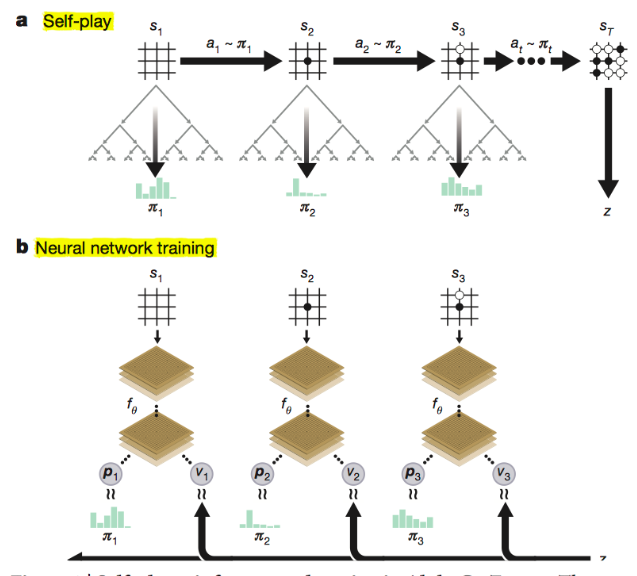
Dual-Headed Neural Network

Network Structure

In AlphaZero, we use a unified dual-headed neural network to simultaneously predict policy and value. This network receives the current board state to compute outputs:

• $p$: A probability distribution output by the policy head, representing the selection probability of each possible action in state $s$. This policy head is combined with MCTS search to generate stronger decisions. • $v$: A scalar output by the value head, representing the predicted value of the current board state $s$ (probability of final victory).

:::assert Although not two independent networks, AlphaZero’s training process can be viewed as a special type of Actor-Critic method, where MCTS acts as the Critic. MCTS evaluates state values through game simulations and generates policy targets used to train the policy network. While the value network also predicts state values, it primarily assists MCTS rather than being directly used for policy gradient updates like a traditional Critic network. :::

import torch
import torch.nn as nn
import torch.nn.functional as F
 
class AlphaZeroNNet(nn.Module):
    def __init__(self, game, args):
        """
        Parameters:
        - game: Game object providing board size and action space size.
        - args: Parameters containing network structure, such as channel count, dropout probability, etc.
        """
        super(AlphaZeroNNet, self).__init__()
        self.board_x, self.board_y = game.getBoardSize()  # Board dimensions
        self.action_size = game.getActionSize()           # Action space size
        self.args = args
 
        # Convolutional layer block
        self.conv_layers = nn.Sequential(
            nn.Conv2d(1, args.num_channels, kernel_size=3, padding=1),
            nn.BatchNorm2d(args.num_channels),
            nn.ReLU(),
            nn.Conv2d(args.num_channels, args.num_channels, kernel_size=3, padding=1),
            nn.BatchNorm2d(args.num_channels),
            nn.ReLU(),
            nn.Conv2d(args.num_channels, args.num_channels, kernel_size=3),
            nn.BatchNorm2d(args.num_channels),
            nn.ReLU(),
            nn.Conv2d(args.num_channels, args.num_channels, kernel_size=3),
            nn.BatchNorm2d(args.num_channels),
            nn.ReLU(),
        )
 
        # Calculate convolutional output size
        conv_output_size = self._get_conv_output_size()
 
        # Fully connected layer block
        self.fc_layers = nn.Sequential(
            nn.Linear(conv_output_size, 1024),
            nn.BatchNorm1d(1024),
            nn.ReLU(),
            nn.Dropout(args.dropout),
            nn.Linear(1024, 512),
            nn.BatchNorm1d(512),
            nn.ReLU(),
            nn.Dropout(args.dropout),
        )
 
        # Policy head: outputs log probabilities for each action
        self.policy_head = nn.Linear(512, self.action_size)
 
        # Value head: outputs value estimate for the current state
        self.value_head = nn.Linear(512, 1)
 
    def _get_conv_output_size(self):
        """
        Calculates the number of features in the convolutional output.
        """
        dummy_input = torch.zeros(1, 1, self.board_x, self.board_y)
        output_feat = self.conv_layers(dummy_input)
        n_size = output_feat.view(1, -1).size(1)
        return n_size
 
    def forward(self, s):
        """
        Forward pass function.
 
        Parameters:
        - s: Input board state, shape (batch_size, board_x, board_y).
 
        Returns:
        - log_policies: Log probabilities of policies, shape (batch_size, action_size).
        - values: Value estimates, shape (batch_size, 1).
        """
        # Adjust input shape
        s = s.view(-1, 1, self.board_x, self.board_y)  # (batch_size, 1, board_x, board_y)
 
        # Extract features with convolutional layers
        s = self.conv_layers(s)  # (batch_size, num_channels, new_board_x, new_board_y)
 
        # Flatten convolutional output
        s = s.view(s.size(0), -1)  # (batch_size, conv_output_size)
 
        # Extract high-level features with fully connected layers
        s = self.fc_layers(s)  # (batch_size, 512)
 
        # Policy head output
        policies = self.policy_head(s)  # (batch_size, action_size)
        log_policies = F.log_softmax(policies, dim=1)
 
        # Value head output
        values = self.value_head(s)  # (batch_size, 1)
        values = torch.tanh(values)  # Limit value to [-1, 1]
 
        return log_policies, values

• Convolutional layers for feature extraction: Multiple layers to extract spatial features of the board.
• Fully connected layers for output: Flatten features and output policy and value respectively.
• Activation functions:
  • log_softmax for policy output to facilitate cross-entropy loss calculation.
  • tanh for value output to limit values between $[-1, 1]$.

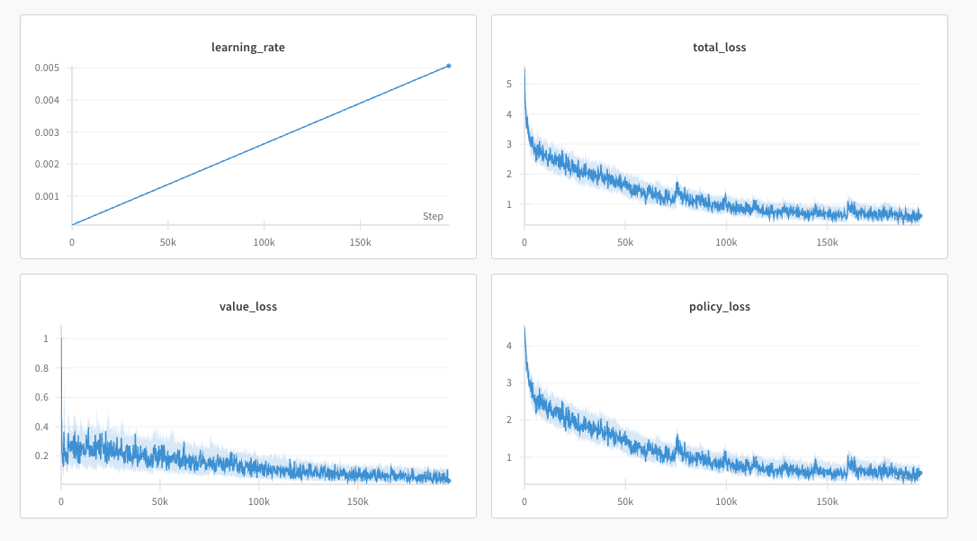
Loss Function

The training goal is implemented through the following loss function to simultaneously train the network’s policy and value estimation capabilities:

• $(z - v)^2$: Value loss, requiring the network output $v$ to be as close as possible to the game result $z$ (+1 for win, -1 for loss, 0 for draw). • $- \pi \log p$: Policy loss, using cross-entropy to require the network output policy $p$ to match the final policy $\pi$ obtained from MCTS as much as possible. • $c \| \theta \|^2$: L2 regularization term to prevent overfitting by keeping the scale of model parameters $\theta$ appropriate.

MCTS Class

class MCTS:
    def __init__(self, game, nnet, args):
        self.game = game         # Game environment
        self.nnet = nnet         # Neural network
        self.args = args         # Parameters
        self.Qsa = {}            # Stores Q values: Q(s,a)
        self.Nsa = {}            # Stores visit counts for edges: N(s,a)
        self.Ns = {}             # Stores visit counts for nodes: N(s)
        self.Ps = {}             # Stores policy priors: P(s,a)
 
        self.Es = {}             # Stores game-over info: E(s)
        self.Vs = {}             # Stores valid moves: V(s)

A highlight here is the caching mechanism: Using dictionaries to cache calculation results, avoiding redundant computation and improving efficiency.

Valid Action Masking

In many games, certain actions are illegal in specific states. For instance, in Gomoku, if a position is already occupied, placing a stone there is illegal. Therefore, ensuring that only legal actions are considered is crucial for algorithm correctness and efficiency. This is achieved through a valid action mask.

In the search method, when we reach a leaf node and need to use the neural network for prediction, we process the policy output from the network using a valid mask to block illegal actions.

if s not in self.Ps: # Not in policy prior store P(s,a)
    # Leaf node, expand based on neural network output policy
    self.Ps[s], v = self.nnet.predict(canonicalBoard)
    valids = self.game.getValidMoves(canonicalBoard, 1)  # Get mask of valid moves, 1 for valid
    self.Ps[s] = self.Ps[s] * valids  # Mask illegal actions
    sum_Ps_s = np.sum(self.Ps[s])
    
    if sum_Ps_s > 0:
        self.Ps[s] /= sum_Ps_s  # Normalize policy probabilities
    else:
        # All actions masked, use uniform distribution
        self.Ps[s] = self.Ps[s] + valids
        self.Ps[s] /= np.sum(self.Ps[s])
 
    self.Vs[s] = valids  # Store mask of valid moves
    self.Ns[s] = 0       # Initialize state visit count
    return v

PUCT

A variation of the UCB formula specifically for MCTS.

In AlphaZero, MCTS uses the neural network output to guide the search direction. During search, the neural network selects actions through the improved upper confidence bound formula PUCT (Polynomial Upper Confidence Trees for Trees), which introduces the prior probability $P(s, a)$. This allows MCTS to use external knowledge (the policy network) to guide the search:

Where:

• $Q(s, a)$ is the average value of selecting action $a$ in state $s$.
• $P(s, a)$ is the prior probability provided by the neural network.
• $N(s)$ and $N(s, a)$ are the visit counts for state $s$ and edge $(s, a)$ respectively.
• $c_{puct}$ is a constant controlling the degree of exploration. Combined with the following exploration term, it encourages choosing actions with fewer visits but high prior probabilities.

cur_best = -float('inf') # Track current max U value
best_act = -1            # Track action with max U value
 
# Traverse all possible actions
for a in range(self.game.getActionSize()):
    if valids[a]: 
        # Calculate PUCT for valid actions
        if (s, a) in self.Qsa:
            # If (s, a) was visited before, use calculated Q value and visit count
            u = self.Qsa[(s, a)] + self.args.cpuct * self.Ps[s][a] * \
                math.sqrt(self.Ns[s]) / (1 + self.Nsa[(s, a)])
        else:
            # If unvisited node, Q value is 0, encouraging exploration
            u = self.args.cpuct * self.Ps[s][a] * math.sqrt(self.Ns[s] + 1e-8) # Give higher U value to unvisited actions, avoiding division by zero
 
        # Select action with highest U value
        if u > cur_best:
            cur_best = u
            best_act = a

Balancing Exploration and Exploitation

• Unvisited nodes have smaller denominators since N(s, a) = 0, making the exploration term larger and encouraging the algorithm to explore new actions.

• $Q(s, a)$ reflects the current estimate of action value, representing exploitation.

Value Inversion

From player $A$’s perspective, higher value for them means lower value for player $B$, and vice versa. Therefore, throughout the search and value evaluation process, value must reflect the maximization of the current player’s interest, maintaining perspective consistency.

In code, this is implemented in calls like:

v = -self.search(next_s)

Search Function

def search(self, canonicalBoard):
    """
    Performs one MCTS search.
 
    Parameters:
    - canonicalBoard: Current player's board state (canonical form)
 
    Returns:
    - v: Value evaluation for the current node
    """
    s = self.game.stringRepresentation(canonicalBoard)
 
    if s not in self.Es:
        self.Es[s] = self.game.getGameEnded(canonicalBoard, 1)
    if self.Es[s] is not None:
        # If game over, return result
        return self.Es[s]
 
    '''
    Valid Mask & Leaf Node Expansion
    '''
 
    valids = self.Vs[s]
 
    '''
    Select optimal action using PUCT formula
    '''
 
    a = best_act
    next_s, next_player = self.game.getNextState(canonicalBoard, 1, a)
    next_s = self.game.getCanonicalForm(next_s, next_player)
 
    # Invert value of next state
    v = -self.search(next_s)
 
    # Update Q value and visit counts
    if (s, a) in self.Qsa:
        self.Qsa[(s, a)] = (self.Nsa[(s, a)] * self.Qsa[(s, a)] + v) / (self.Nsa[(s, a)] + 1)
        self.Nsa[(s, a)] += 1
    else:
        self.Qsa[(s, a)] = v
        self.Nsa[(s, a)] = 1
 
    self.Ns[s] += 1
    return v

• Recursive search simulates future possibilities.
• Leaf node prediction with neural networks speeds up search.
• Value inversion due to alternating players.

Self-Play

A Go algorithm trained without human game data, obtaining data solely through self-play.

Self-play means for every move, multiple MCTS iterations are executed to get an improved policy $\pi(s,a)$ for move selection. Players alternate black and white stones until the game ends. Self-play generates massive training data, helping the neural network learn better policies and value estimates.

Executing an Episode of Self-Play

Let’s look at the core function of Self-Play: executeEpisode, which executes a full game until it ends and collects training data.

def executeEpisode(self):
    """
    Executes an episode of self-play and returns a list of training samples.
 
    Returns:
        trainExamples: A list containing multiple (canonicalBoard, pi, v) tuples.
    """
    trainExamples = []
    board = self.game.getInitBoard()  # Initialize board
    self.curPlayer = 1                # Current player (1 or -1)
    episodeStep = 0                   # Record step count
 
    while True: # Until game over
        episodeStep += 1
        canonicalBoard = self.game.getCanonicalForm(board, self.curPlayer)
 
        temp = int(episodeStep < self.args.tempThreshold)  # Temperature parameter
 
        pi = self.mcts.getActionProb(canonicalBoard, temp=temp)  # Use MCTS to get policy
        sym = self.game.getSymmetries(canonicalBoard, pi)        # Data augmentation (symmetries)
        for b, p in sym:
            trainExamples.append([b, self.curPlayer, p, None])
 
        action = np.random.choice(len(pi), p=pi)  # Choose action based on policy probabilities
        board, self.curPlayer = self.game.getNextState(board, self.curPlayer, action) # Execute action, update board and player. 
 
        r = self.game.getGameEnded(board, self.curPlayer)  # Check if game over
        if r is not None:
            # Assign final value to each sample: +1 for winner, -1 for loser, 0 for draw
            return [(x[0], x[2], r * ((-1) ** (x[1] != self.curPlayer))) for x in trainExamples]

• Temperature Parameter: Controls policy exploration. Set to 1 early on to encourage exploration; set to 0 later to bias towards exploitation of optimal strategies.

• Data Augmentation: In Gomoku, board rotation and flipping do not change the essence of the game. Using these symmetries generates equivalent boards and policies, increasing training data to improve model generalization.

When the game ends, training samples are generated from the game log and returned in trainExamples.

Main Self-Play Loop

Self-play isn’t just one game; we need to continuously perform self-play and update the model across multiple iterations.

def learn(self):
    """
    Performs multiple iterations of self-play and model updates.
    """
    for i in range(1, self.args.numIters + 1):
        log.info(f"Starting Iter #{i} ...")
        # Store training samples for this iteration
        iterationTrainExamples = deque([], maxlen=self.args.maxlenOfQueue)
 
        # Perform specified number of self-play episodes
        for _ in tqdm(range(self.args.numEps), desc="Self Play"):
            self.mcts = MCTS(self.game, self.nnet, self.args)  # Reset MCTS
            iterationTrainExamples += self.executeEpisode()
 
        # Save training samples
        self.trainExamplesHistory.append(iterationTrainExamples)
 
        # Maintain fixed length training history
        if len(self.trainExamplesHistory) > self.args.numItersForTrainExamplesHistory:
            log.warning(f"Removing the oldest entry in trainExamples.")
            self.trainExamplesHistory.pop(0)
 
        # Combine and shuffle all training samples
        trainExamples = []
        for e in self.trainExamplesHistory:
            trainExamples.extend(e)
        shuffle(trainExamples)
 
        # Train neural network
        self.nnet.save_checkpoint(folder=self.args.checkpoint, filename="temp.pth.tar")
        self.pnet.load_checkpoint(folder=self.args.checkpoint, filename="temp.pth.tar")
        pmcts = MCTS(self.game, self.pnet, self.args)
 
        self.nnet.train(trainExamples)
        nmcts = MCTS(self.game, self.nnet, self.args)

• If history exceeds a threshold, oldest samples are removed to prevent overfitting to old data.
• After collecting enough data, the model is trained with self.nnet.train(trainExamples).

Filtering Mechanism

To ensure the model’s strength continuously improves, AlphaGo Zero introduced a filtering mechanism for pitting new models against old ones:

• After each training round, the new model plays against the old one.
  • If the new model’s win rate exceeds a threshold (e.g., 55%), it’s accepted for the next round of self-play; otherwise, the old model’s weights are restored, and data generation/training continues from there to avoid meaningless regression and overfitting.

        # Evaluate new model
        log.info("PITTING AGAINST PREVIOUS VERSION")
        arena = game.Arena(lambda x: np.argmax(pmcts.getActionProb(x, temp=0)),
                           lambda x: np.argmax(nmcts.getActionProb(x, temp=0)),
                           self.game)
        pwins, nwins, draws = arena.playGames(self.args.arenaCompare)
 
        log.info(f"NEW/PREV WINS : {nwins} / {pwins} ; DRAWS : {draws}")
        if pwins + nwins == 0 or float(nwins) / (pwins + nwins) < self.args.updateThreshold:
            log.info("REJECTING NEW MODEL")
            self.nnet.load_checkpoint(folder=self.args.checkpoint, filename="temp.pth.tar")
        else:
            log.info("ACCEPTING NEW MODEL")
            self.nnet.save_checkpoint(folder=self.args.checkpoint, filename="best.pth.tar")

Getting Policy from MCTS

During self-play, we use MCTS to choose actions. getActionProb obtains policy probabilities from MCTS.

def getActionProb(self, canonicalBoard, temp=1):
    """
    Performs multiple MCTS searches and returns action probability distribution.
 
    Parameters:
        canonicalBoard: Current canonical board state
        temp: Temperature parameter
 
    Returns:
        probs: Action probability distribution
    """
    # Perform specified number of MCTS searches
    for _ in range(self.args.numMCTSSims):
        self.search(canonicalBoard) 
 
    s = self.game.stringRepresentation(canonicalBoard)
    # Record visit count N(s, a) for each action
    counts = [self.Nsa[(s, a)] if (s, a) in self.Nsa else 0 
              for a in range(self.game.getActionSize())]
 
    if temp == 0:
        bestAs = np.array(np.argwhere(counts == np.max(counts))).flatten()
        bestA = np.random.choice(bestAs)
        probs = [0] * len(counts)
        probs[bestA] = 1
        return probs
 
    counts = [x ** (1. / temp) for x in counts]
    counts_sum = float(sum(counts))
    probs = [x / counts_sum for x in counts]
    return probs

Visit counts N(s, a) reflect MCTS’s confidence in an action.

Calculating Policy Probabilities:

• When temp = 0:
  • Chooses the action with the most visits, probability 1.
  • Ensures policy determinism, usually for late game or evaluation.
• When temp > 0:
  • Temperature transform on visit counts: counts = [x ** (1. / temp) for x in counts].
  • Higher temperature means policy is closer to uniform distribution, stronger exploration.

Training Journey

MCTS simulations: 400, cpuct: 1.0, 50 iterations:

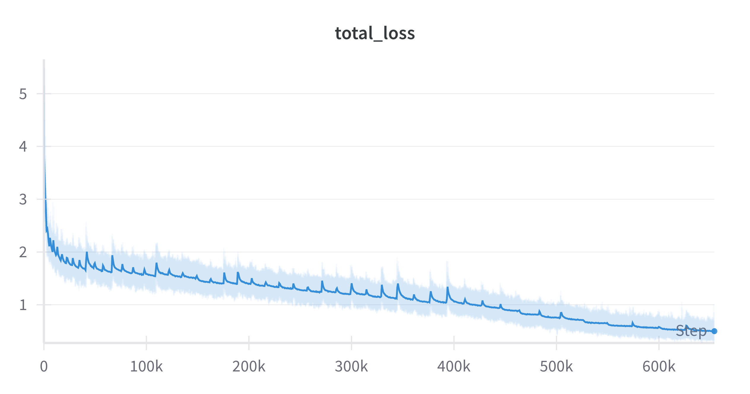
By this point, the model has learned the rules of Gomoku, reaching basic difficulty. You can win by sneaking moves near the edge.

Adding 1cycle Learning Rate Adjustment

Dynamic learning rate adjustment can improve convergence speed and generalization.

• Phase 1 (First half): Learning rate gradually increases from minimum ($1.0 \times 10^{-4}$) to maximum ($1.0 \times 10^{-2}$).
• Phase 2 (Second half): Learning rate gradually decreases back to minimum.

class NNetWrapper:
    def __init__(self, game, args):
        ... # other initializations
        self.optimizer = optim.Adam(self.nnet.parameters(), lr=args.max_lr)
        
        # 1cycle LR parameters
        self.total_steps = args.numIters * args.epochs * (args.maxlenOfQueue // args.batch_size)
        self.current_step = 0
 
    def get_learning_rate(self):
        """Implements 1cycle learning rate policy"""
        if self.current_step >= self.total_steps:
            return self.args.min_lr
        
        half_cycle = self.total_steps // 2
        
        if self.current_step <= half_cycle:
            # Phase 1: Increase from min_lr to max_lr
            phase = self.current_step / half_cycle
            lr = self.args.min_lr + (self.args.max_lr - self.args.min_lr) * phase
        else:
            # Phase 2: Decrease from max_lr to min_lr
            phase = (self.current_step - half_cycle) / half_cycle
            lr = self.args.max_lr - (self.args.max_lr - self.args.min_lr) * phase
        
        return lr

Adding Gradient Clipping

Can review PPO for this.

To prevent gradient explosion and stabilize training, we add gradient clipping after backpropagation. Assuming the gradient vector for some parameter is $\mathbf{g}$, and its current L2 norm is $\|\mathbf{g}\|$:

• If $\|\mathbf{g}\| \leq 1.0$, then $\mathbf{g}$ remains unchanged.
• If $\|\mathbf{g}\| > 1.0$, then $\mathbf{g}$ is scaled to $\frac{1.0}{\|\mathbf{g}\|} \cdot \mathbf{g}$.

This ensures:

def train(self, examples):
    ... # other training steps
    for epoch in range(self.args.epochs):
        ... # iterate through batches
        for _ in t:
            ... # forward pass and loss calculation
            total_loss.backward()
 
            # Gradient clipping
            if self.args.grad_clip:
                torch.nn.utils.clip_grad_norm_(self.nnet.parameters(), self.args.grad_clip)
 
            # Update parameters
            self.optimizer.step()
            ... # update learning rate, etc.

Gradient clipping limits the norm of gradients within a threshold, preventing large gradients from destabilizing training. By clipping before each parameter update, we ensure training robustness and accelerate convergence.

Conclusion

Final code and demos can be found in the repository below, and model weights are available in the Hugging Face links within the documentation.

https://github.com/Nagi-ovo/alphazero-gomoku

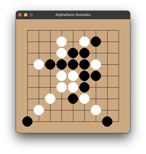
After these improvements, increasing MCTS simulations to 2000 and cpuct to 4.0 for stronger exploration, and training for 22 iterations (running for 4 days on a single 3090 Ti), our model upgraded to normal difficulty. (At 50 MCTS simulations, the early game pressure is decent, but it might miss the opponent’s winning points in the mid-to-late game).

Increasing MCTS simulations during inference can bring it to hard difficulty. Try and see if you can win if you’re interested.

References

• Zhihu Sunrise: Understanding AlphaZero from Scratch, MCTS, Self-Play, UCB
• AlphaZero Explained · On AI
• Part 1: How to Train a Gomoku Robot using Self-Play RL - Alpha Gobang Zero